Profile Maximum Likelihood: An Optimal, Universal, Plug-and-Play - PowerPoint PPT Presentation

Profile Maximum Likelihood: An Optimal, Universal, Plug-and-Play Functional Estimator Yi Hao and Alon Orlitsky, UCSD 0 / 19

Outline Property estimation Plug-in estimators Prior results Profile maximum likelihood Results Simple, unified, optimal, plug-in, estimators for four learning tasks Proof elements: The fun theorem of maximum likelihood Local heroes 1 / 19

Discrete Distributions Discrete support set X { heads, tails } = { h, t } { ..., − 1 , 0 , 1 ,... } = Z Distribution p over X , probability p x for x ∈ X p x ≥ 0 ∑ x ∈X p x = 1 p = ( p h ,p t ) p h = . 6 , p t = . 4 P collection of distributions P X all distributions over X P { h, t } = {( p h ,p t )} = {( . 6 ,. 4 ) , ( . 4 ,. 6 ) , ( . 5 ,. 5 ) , ( 0 , 1 ) ,... } 2 / 19

Distribution Functional f ∶ P X → R Maps distribution to real value H ( p ) ∑ x p x log 1 Shannon entropy p x H α ( p ) 1 − α log ( ∑ x p α x ) 1 Rényi entropy S ( p ) Support size ∑ x 1 p x > 0 S m ( p ) ∑ x ( 1 − ( 1 − p x ) m ) Support coverage Expected # distinct symbols in m samples L uni ( p ) ∑ x ∣ p x − 1 ∣X∣ ∣ Distance to uniformity max ( p ) max { p x ∶ x ∈ X} Highest probability ... Many applications 3 / 19

Property Estimation Given: support set X , property f Unknown: p ∈ P X Estimate: f ( p ) Entropy of English words Given: X = { English words } , estimate: H ( p ) unknown: p , # species in habitat Given: X = { bird species } , estimate: S ( p ) unknown: p , How to estimate f ( p ) when p is unknown? 4 / 19

Learn from Examples Observe n independent samples X n = X 1 ,...,X n ∼ p Reveal information about p Estimate f ( p ) Estimator: f est ∶ X n → R Estimate for f ( p ) : f est ( X n ) Simplest estimators? 5 / 19

Plug-in Estimators Simple two-step estimators Use X n to derive estimate p est ( X n ) of p Plug-in f ( p est ( X n )) to estimate f ( p ) Hope: As n → ∞ , p est ( X n ) → p , then f ( p est ( X n )) → f ( p ) Simplest p est ? 6 / 19

Empirical Estimator n samples N x # times x appears ∶ = N x p emp x n X = { a,b,c } p = ( p a ,p b ,p c ) = ( . 5 ,. 3 ,. 2 ) Estimate p from n = 10 samples X 10 = c,a,b,a,b,a,b,a,b,c p emp p emp 4 4 p emp 2 = = = 10 , 10 , a c b 10 p emp = ( . 4 ,. 4 ,. 2 ) 7 / 19

Empirical Plug-In Estimator f emp ( X n ) = f ( p emp ( X n )) Entropy estimation X 10 = c,a,b,a,b,a,b,a,b,c p emp = ( . 4 ,. 4 ,. 2 ) H emp ( X 10 ) ∶ = H ( . 4 ,. 4 ,. 2 ) Advantages Plug-and-play: simple two steps Universal: applies to all properties Intuitive Best-known, most-used distribution estimator Performance? 8 / 19

Sample Complexity Min-max Probably Approximately Correct (PAC) Formulation Allowed additive approximation error ǫ > 0 Allowed error probability δ > 0 n f ( f est ,p,ε,δ ) : # samples f est needs to approximate f well, ∣ f est ( X n ) − f ( p )∣ ≤ ε with probability ≥ 1 − δ n f ( f est , P ,ε,δ ) ∶ = max p ∈P n f ( f est ,p,ε,δ ) : # samples f est needs to approximate every p ∈ P n f (P ,ε,δ ) ∶ = min f est n f ( f est , P ,ε,δ ) # samples the best estimator needs to approximate all distributions in P 9 / 19

Empirical and Optimal Sample Complexity ∣X∣ = k , P X ∣ all distributions n f ( f emp ,ε, 1 / 3 ) n f ( ε, 1 / 3 ) Property k k ⋅ 1 log k ⋅ 1 Entropy ε ε log m ⋅ log 1 m Supp. coverage m ε k ⋅ 1 log k ⋅ 1 k Dist. to uniform ε 2 ε 2 k ⋅ log 1 log k ⋅ log 2 1 k Support size ε ε P03, VV11a/b, WY14/19, JVHW14/18, AOST14, OSW16, ADOS17, PW 19,. . . For support size, P ≥ 1 / k ∶ = { p ∣ p x ≥ 1 / k, ∀ x ∈ X} Regime where ε ≳ n − 0 . 1 Support size and coverage normalized by k and m respectively Why is empirical plugin good? suboptimal? optimal plug-in? 10 / 19

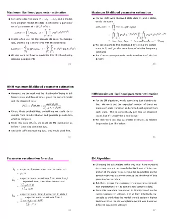
Maximum Likelihood i.i.d. p ∈ P X , probability of observing x n ∈ X n p ( x n ) ∶ = Pr X n ∼ p ( X n = x n ) = ∏ n i = 1 p ( x i ) Maximum likelihood estimator: x n → dist. p maximizing p ( x n ) p ml ( x n ) = arg max p p ( x n ) p ml ( h,t,h ) = arg max p h + p t = 1 p 2 h ⋅ p t p h = 2 / 3 , p t = 1 / 3 Identical to empirical estimator – always Empirical good: Distribution that best explains observation Work wells for small alphabets large sample Overfits data when alphabet is large relative to sample size Improve? 11 / 19

What Counts iid: Do not care about order Entropy, Rényi, support size, coverage: symmetric functionals Do not care about labels (h,h,t), (t,t,h), (h,t,h), (t,h,t), (t,h,h), (h,t,t) same entropy Care only: # of elements appearing any given number of times Three samples: 1 element appeared once, 1 element appeared twice Profile: ϕ = { 1 , 2 } 12 / 19

Profile maximum likelihood (PML) Profile ϕ ( x n ) of x n is the multiset of symbol frequencies bananas � ⇒ a appears thrice, n twice, bs once � ⇒ ϕ ( bananas ) = { 3 , 2 , 1 , 1 } Probability of observing a profile ϕ when sampling from p is n p ( ϕ ) ∶ = p ( y n ) = p ( y i ) ∑ ∑ ∏ i = 1 y n ∶ ϕ ( y n )= ϕ y n ∶ ϕ ( y n )= ϕ Profile maximum likelihood maps x n to ϕ ( x n ) ∶ = argmax p ( ϕ ( x n )) p ml p ∈P X 13 / 19

Simple Profile ML Observe x 3 = h,t,h Sequence ML: p h = 2 / 3 , p t = 1 / 3 Profile: ϕ = { 1 , 2 } Profile ML: maximize probability of ϕ = { 1 , 2 } p + q = 1 p,q Pr ( ϕ = { 1 , 2 }) = ppq + qqp + pqp + qpq + qpp + pqq = 3 ( p 2 q + q 2 p ) max ( p 2 q + q 2 p ) = max ( qp ⋅ ( p + q )) = max pq Profile ML: p = q = 1 2 More logical More interesting? 14 / 19

RESULTS 15 / 19

Summary Profile maximum likelihood (PML) is a unified, time- and sample-optimal approach to four basic learning problems Additive property estimation Rényi entropy estimation Sorted distribution estimation Uniformity testing Yi Hao and Alon Orlitsky The Broad Optimality of Profile Maximum Likelihood Arxiv, NeurIPS 2019 16 / 19

Additive Functional Estimation Additive functional: f ( p ) = ∑ x f ( p x ) Entropy, support size, coverage, distance to uniformity For all symmetric, additive, Lipschitz ∗ , functionals, for n ≥ n f (∣X∣ ,ε, 1 / 3 ) and ε ≥ n − 0 . 1 , ϕ ( X 4 n ) ) − f ( p )∣ > 5 ε ) ≤ exp (−√ n ) Pr (∣ f ( p ml With four times the optimal # samples for error probability 1 / 3 , PML plug-in achieves much lower error probability Covers four functionals above Can use near-linear-time PML approximation [CSS19] 17 / 19

Additional results Rényi Entropy For integer α > 1 , PML plug-in has optimal k 1 − 1 / α sample complexity For non-integer α > 3 / 4 , (A)PML plug-in improves best-known results Sorted Distribution Estimation Under ℓ 1 distance, (A)PML yields optimal Θ ( k /( ε 2 log k )) sample complexity for sorted distribution estimation Actual distribution in ℓ 1 distance, 2 ( k − 1 )/( πε 2 ) [KOPS ’15] √ Uniformity testing : p = p u v.s. ∣ p − p u ∣ ≥ ε ; complexity Θ ( k / ε 2 ) Tester below is sample-optimal up to logarithmic factors of k Input: parameters k,ε, and a sample X n ∼ p with profile ϕ If any symbol appears ≥ 3max { 1 ,n / k } log k times, return 1 √ If ∣∣ p ml ϕ − p u ∣∣ 2 ≥ 3 ε /( 4 k ) , return 1 ; else, return 0 18 / 19

Thank you! 19 / 19