Lecture 3. Inadmissibility of Maximum Likelihood Estimate and - PowerPoint PPT Presentation
Lecture 3. Inadmissibility of Maximum Likelihood Estimate and James-Stein Estimator Yuan Yao Hong Kong University of Science and Technology March 4, 2020 Outline Recall: PCA in Noise Maximum Likelihood Estimate Example: Multivariate Normal
Lecture 3. Inadmissibility of Maximum Likelihood Estimate and James-Stein Estimator Yuan Yao Hong Kong University of Science and Technology March 4, 2020
Outline Recall: PCA in Noise Maximum Likelihood Estimate Example: Multivariate Normal Distribution James-Stein Estimator Risk and Bias-Variance Decomposition Inadmissability James-Stein Estimators Stein’s Unbiased Risk Estimates (SURE) Proof of SURE Lemma Recall: PCA in Noise 2
PCA in Noise ◮ Data: x i ∈ R p , i = 1 , . . . , n ◮ PCA looks for Eigen-Value Decomposition (EVD) of sample covariance matrix: � n Σ n = 1 ˆ µ n ) T ( x i − ˆ µ n )( x i − ˆ n i =1 where � n µ n = 1 ˆ x i n i =1 ◮ Geometric view as the best affine space approximation of data ◮ What about statistical view when x i = µ + ε i ? Recall: PCA in Noise 3
Recall: Phase Transitions of PCA For rank-1 signal-noise model α ∼ N (0 , σ 2 X = αu + ε, X ) , ε ∼ N (0 , I p ) PCA undergoes a phase transition if p/n → γ : ◮ The primary eigenvalue of sample covariance matrix satisfies � (1 + √ γ ) 2 = b, X ≤ √ γ σ 2 λ max ( � Σ n ) → (1) X > √ γ γ (1 + σ 2 σ 2 X )(1 + X ) , σ 2 ◮ The primary eigenvector converges to X ≤ √ γ σ 2 0 |� u, v max �| 2 → γ 1 − (2) X > √ γ σ 4 σ 2 , X γ 1+ σ 2 X Recall: PCA in Noise 4
Recall: Phase Transitions of PCA ◮ Here the threshold p γ = lim n n,p →∞ ◮ The law of large numbers in traditional statistics assumes p fixed and n → ∞ : γ = lim n →∞ p/n = 0 . where PCA always works without phase transitions. ◮ In high dimensional statistics , we allow both p and n grow: p, n → ∞ , not law of large numbers. ◮ What might go wrong? Even the sample mean ˆ µ n ! Recall: PCA in Noise 5
In this lecture µ n and covariance ˆ ◮ Sample mean ˆ Σ n are both Maximum Likelihood Estimate (MLE) under Gaussian noise models ◮ In high dimensional scenarios (small n , large p ), MLE ˆ µ n is not optimal: – Inadmissability: MLE has worse prediction power than James-Stein Estimator (JSE) (Stein, 1956) – Many shrinkage estimates are better than MLE and James-Stein Estimator (JSE) ◮ Therefore, penalized likelihood or regularization is necessary in high dimensional statistics Recall: PCA in Noise 6
Outline Recall: PCA in Noise Maximum Likelihood Estimate Example: Multivariate Normal Distribution James-Stein Estimator Risk and Bias-Variance Decomposition Inadmissability James-Stein Estimators Stein’s Unbiased Risk Estimates (SURE) Proof of SURE Lemma Maximum Likelihood Estimate 7
Maximum Likelihood Estimate ◮ Statistical model f ( X | θ ) as a conditional probability function on R p with parameter space θ ∈ Θ ◮ The likelihood function is defined as the probability of observing the given data x i ∼ f ( X | θ ) as a function of θ , n � L ( θ ) = f ( x i | θ ) i =1 ◮ A Maximum Likelihood Estimator is defined as n � ˆ θ MLE ∈ arg max θ ∈ Θ L ( θ ) = arg max f ( x i | θ ) n θ ∈ Θ i =1 n � 1 = arg max log f ( x i | θ ) . (3) n θ ∈ Θ i =1 Maximum Likelihood Estimate 8
Maximum Likelihood Estimate ◮ For example, consider the normal distribution N ( µ, Σ) , � � 1 − 1 2( X − µ ) T Σ − 1 ( X − µ ) f ( X | µ, Σ) = � exp , (2 π ) p | Σ | where | Σ | is the determinant of covariance matrix Σ . ◮ Take independent and identically distributed (i.i.d.) samples x i ∼ N ( µ, Σ) ( i = 1 , . . . , n ) Maximum Likelihood Estimate 9
Maximum Likelihood Estimate (continued) ◮ To get the MLE given x i ∼ N ( µ, Σ) ( i = 1 , . . . , n ) , solve n n � � 1 exp[ − ( X i − µ ) T Σ − 1 ( X i − µ )] max f ( x i | µ, Σ) = max � 2 π | Σ | µ, Σ µ, Σ i =1 i =1 ◮ Equivalently, consider the logarithmic likelihood n � J ( µ, Σ) = log f ( x i | µ, Σ) i =1 n � − 1 ( X i − µ ) T Σ − 1 ( X i − µ ) − n = 2 log | Σ | + C (4) 2 i =1 where C is a constant independent to parameters Maximum Likelihood Estimate 10
MLE: sample mean ˆ µ n ◮ To solve µ , the log-likelihood is a quadratic function of µ , � n � � 0 = ∂J � Σ − 1 ( x i − µ ∗ ) µ = µ ∗ = − � ∂µ i =1 � n ⇒ µ ∗ = 1 x i = ˆ µ n n i =1 Maximum Likelihood Estimate 11
MLE: sample covariance ˆ Σ n ◮ To solve Σ , the first term in (4) n � − 1 Tr ( x i − µ ) T Σ − 1 ( x i − µ ) 2 i =1 n � − 1 Tr [Σ − 1 ( x i − µ )( x i − µ ) T ] , = Tr ( ABC ) = Tr ( BCA ) 2 i =1 n � − n Σ n := 1 2 ( Tr Σ − 1 ˆ µ n ) T , ˆ = Σ n ) , ( x i − ˆ µ n )( x i − ˆ n i =1 − n 1 1 2 Tr (Σ − 1 ˆ n ˆ = Σ 2 Σ n ) 2 − n n Σ − 1 ˆ 1 1 2 Tr (ˆ = Σ Σ n ) , Tr ( ABC ) = Tr ( BCA ) 2 2 − n 1 1 n Σ − 1 ˆ S := ˆ = 2 Tr ( S ) , Σ 2 Σ 2 n Maximum Likelihood Estimate 12
MLE: sample covariance ˆ Σ n Use S to represent Σ : ◮ Notice that n S − 1 ˆ 1 1 Σ = ˆ Σ Σ 2 2 n ⇒ − n 2 log | Σ | = n 2 log | S | + n 2 log | ˆ Σ n | = f (ˆ Σ n ) where we use for determinant of squared matrices of equal size, det( AB ) = | AB | = det( A ) det( B ) = | A | · | B | . ◮ Therefore, n 2 Tr ( S ) − n 2 log | S | + Const (ˆ max J (Σ) ⇔ min Σ n , 1) Σ S Maximum Likelihood Estimate 13
MLE: sample covariance ˆ Σ n 1 1 n Σ − 1 ˆ ◮ Since S = ˆ Σ 2 Σ n is symmetric and positive semidefinite, let 2 S = U Λ U T be its eigenvalue decomposition, Λ = diag ( λ i ) with λ 1 ≥ λ 2 ≥ . . . ≥ λ p ≥ 0 . Then we have p p � � J ( λ i ) = n λ i − n log( λ i ) + Const 2 2 i =1 i =1 � � ⇒ 0 = ∂J = n 2 − n 1 � ⇒ λ ∗ i = 1 � λ ∗ ∂λ i 2 λ ∗ i i ⇒ S ∗ = I p ◮ Hence the MLE solution n � Σ n = 1 Σ ∗ = ˆ µ n ) T , ( X i − ˆ µ n )( X i − ˆ n i =1 Maximum Likelihood Estimate 14
Note ◮ In statistics, it is often defined � n 1 µ n ) T , ˆ ( X i − ˆ µ n )( X i − ˆ Σ n = n − 1 i =1 where the denominator is ( n − 1) instead of n . This is because that for sample covariance matrix, a single sample n = 1 leads to no variance at all. Maximum Likelihood Estimate 15
Consistency of MLE Under some regularity conditions, the maximum likelihood estimator ˆ θ MLE has the following nice limit properties for fixed p and n → ∞ : n A. (Consistency) ˆ θ MLE → θ 0 , in probability and almost surely. n B. (Asymptotic Normality) √ n (ˆ − θ 0 ) → N (0 , I − 1 θ MLE 0 ) in n distribution, where I 0 is the Fisher Information matrix ∂θ log f ( X | θ 0 )) 2 ] = − E [ ∂ 2 I ( θ 0 ) := E [( ∂ ∂θ 2 log f ( X | θ 0 )] . C. (Asymptotic Efficiency) lim n →∞ cov(ˆ θ MLE ) = I − 1 ( θ 0 ) . Hence n ˆ θ MLE is the Uniformly Minimum-Variance Unbiased Estimator , n i.e. the estimator with the least variance among the class of unbiased estimators, for any unbiased estimator ˆ θ n , lim n →∞ var(ˆ ) ≤ lim n →∞ var(ˆ θ MLE θ n ) . n Maximum Likelihood Estimate 16
However, large p small n ? ◮ The asymptotic results all hold under the assumption by fixing p and µ n → µ and ˆ taking n → ∞ , where MLE satisfies ˆ Σ n → Σ . ◮ However, when p becomes large compared to finite n , ˆ µ n is not the best estimator for prediction measured by expected mean squared error from the truth, to to shown below. Maximum Likelihood Estimate 17
Outline Recall: PCA in Noise Maximum Likelihood Estimate Example: Multivariate Normal Distribution James-Stein Estimator Risk and Bias-Variance Decomposition Inadmissability James-Stein Estimators Stein’s Unbiased Risk Estimates (SURE) Proof of SURE Lemma James-Stein Estimator 18
Prediction Error and Risk ◮ To measure the prediction performance of an estimator ˆ µ n , it is natural to consider the expected squared loss in regression, i.e. given a response y = µ + ǫ with zero mean noise E [ ǫ ] = 0 , µ n � 2 = E � µ − ˆ µ + ǫ � 2 = E � µ − ˆ Var ( ǫ ) = E ( ǫ T ǫ ) . µ � 2 + Var ( ǫ ) , E � y − ˆ ◮ Since Var ( ǫ ) is a constant for all estimators ˆ µ , one may simply look at the first part which is often called as risk in literature, µ � 2 R (ˆ µ, µ ) = E � µ − ˆ It is the mean square error (MSE) between µ and its estimator ˆ µ , that measures the expected prediction error. James-Stein Estimator 19
Bias-Variance Decomposition ◮ The risk or MSE enjoy the following important bias-variance decomposition , as a result of the Pythagorean theorem. µ n ] − µ � 2 R (ˆ µ n , µ ) = E � ˆ µ n − E [ˆ µ n ] + E [ˆ µ n ] � 2 + � E [ˆ µ n ] − µ � 2 = E � ˆ µ n − E [ˆ µ n ) 2 =: Var (ˆ µ n ) + Bias (ˆ ◮ Consider multivariate Gaussian model, x 1 , . . . , x n ∼ N ( µ, σ 2 I p ) ( i = 1 , . . . , n ), and the maximum likelihood estimators (MLE) of the parameters ( µ and Σ = σ 2 I p ) James-Stein Estimator 20
Example: Bias-Variance Decomposition of MLE ◮ Consider multivariate Gaussian model, Y 1 , . . . , Y n ∼ N ( µ, σ 2 I p ) ( i = 1 , . . . , n ), and the maximum likelihood estimators (MLE) of the parameters ( µ and Σ = σ 2 I p ) ◮ The MLE estimator satisfies µ MLE Bias (ˆ ) = 0 n and ) = p µ MLE nσ 2 Var (ˆ n µ MLE = Y . µ MLE ) = σ 2 p for ˆ In particular for n = 1 , Var (ˆ James-Stein Estimator 21
Recommend
More recommend
Explore More Topics
Stay informed with curated content and fresh updates.
