Synthesizing Probabilistic Invariants via Doobs decomposition G. - PowerPoint PPT Presentation
Synthesizing Probabilistic Invariants via Doobs decomposition G. Barthe, T. Espitau , L.M.F Fioriti, J. Hsu CAV, 2016 Introduction 1 Introduction Probabilistic 1 2 Computations Ubiquitous in many fields (ML, Crypto, Privacy,)
Synthesizing Probabilistic Invariants via Doob’s decomposition G. Barthe, T. Espitau , L.M.F Fioriti, J. Hsu CAV, 2016
Introduction 1
Introduction Probabilistic 1 2 Computations Ubiquitous in many fields (ML, Crypto, Privacy,…) But… Difficult to prove Termination ? (Certainly, almost sure, non terminating)
Introduction Probabilistic Doob’s 1 2 3 Martingales? Computations Decomposition Ubiquitous in many fields Difficulty to transfer local to (ML, Crypto, Privacy,…) end of program But… Difficult to prove Reason on average values Termination ? Martingales have the required (Certainly, almost sure, non transfer property terminating)
Introduction Probabilistic Doob’s 1 2 3 Martingales? Computations Decomposition Ubiquitous in many fields Difficulty to transfer local to But ( again )… Difficult to find (ML, Crypto, Privacy,…) end of program good ones But… Difficult to prove Reason on average values Automated generation? Doob’s decomposition Termination ? Martingales have the required Formal method to generate (Certainly, almost sure, non transfer property martingales from a seed . terminating)
Martingale theory 101 (I)
Martingale theory 101 (I) Step 1: Some probabilities ● Ω set of outcomes. Sigma algebra: Probability space ● Set F of subsets of Ω Closed under complements, countable unions, countable intersections. ● Probability measure: Countably additive mapping P : F → [0, 1] P (Ω) = 1.
Martingale theory 101 (II) Step 2: Stochastic process ● Random variable: X : Ω → R measurable ( X -1 ( (a,b] ) ∈ F ) Filtration: ( F i ) ⊂ F s.t: ● F i-1 ⊂ F i ● Process wrt filtration F i : Sequence (X i ) s.t: X i is F i measurable
Martingale theory 101 (II) Interlude: PL setting i = 0 Ω: Element = Possible outcome of samples While b do z[i] ← $ Samplings... F i : Events sampled at iteration i or before x[i] ← f(x[i-1], ... , f[0], z[i], … ,z[0]) i++ end Process (X i ) is adapted to the filtration iff: X i is defined in term of elements sampled at step i or before
Martingale theory 101 (III) Step 3: Expectations & Moments ● Expectation: E [X] = ∑ u ∈ Ω X(u) P (u) Conditional expectation wrt G ⊂ F: E [X|G] ● Y G-mesurable st E [X. 1 A ] = E [Y. 1 A ] for A ∈ G
Martingale theory 101 (IV) Step 4 ( Final! ): Martingales Martingale: ● E [ X i | F i-1 ] = X i-1 Average value of the current step is equal to the value of the previous step
Playing with martingales Doob’s decomposition (X i ) stochastic process → (M i ) martingale M 0 = X 0 M i = X 0 + ∑ i j=1 X j - E [X j | F j-1 ]
Black Magic of martingales Optional Stopping theorem (M i ) martingale → Expectations are invariants E [M j ] = E [M 0 ]
Black Magic of martingales Optional Stopping theorem E [M j ] = E [M 0 ]
Black Magic of martingales Optional Stopping theorem E [M T ] = E [M 0 ] For T a stopping time : T : Ω → R { w ∈ Ω | T(w) ≤ i } ⊂ F i
Black Magic of martingales Optional Stopping theorem E [M T ] = E [M 0 ] For T a stopping time : T : Ω → R { w ∈ Ω | T(w) ≤ i } ⊂ F i and... |M i - M i-1 | ≤ C E [T] < ∞
Let’s play with a program...
Geometric distribution x[0] ← 0; while (z ̸ = 0) do z ← $ Bern(p, {1, 0}); x ← x[-1] + z; end
Geometric distribution Stopping time? (on average) x[0] ← 0; while (z ̸ = 0) do z ← $ Bern(p, {1, 0}); x ← x[-1] + z; end
Geometric distribution Stopping time? (on average) x[0] ← 0; while (z ̸ = 0) do 1/(1-p) z ← $ Bern(p, {1, 0}); x ← x[-1] + z; end
Geometric distribution Equation for x ? X i = X i-1 + Z i x[0] ← 0; while (z ̸ = 0) do z ← $ Bern(p, {1, 0}); x ← x[-1] + z; end
Geometric distribution Equation for x ? X i = X i-1 + Z i x[0] ← 0; while (z ̸ = 0) do z ← $ Bern(p, {1, 0}); Polynomial extraction x ← x[-1] + z; end
Geometric distribution X i = X i-1 + Z i x[0] ← 0; while (z ̸ = 0) do M 0 = X 0 M i = X 0 + ∑ i z ← $ Bern(p, {1, 0}); j=1 X j - E [X j | F j-1 ] x ← x[-1] + z; end Doob
Geometric distribution X i = X i-1 + Z i x[0] ← 0; while (z ̸ = 0) do M 0 = 0 M i = X 0 + ∑ i z ← $ Bern(p, {1, 0}); j=1 X j - E [X j | F j-1 ] x ← x[-1] + z; end
Geometric distribution X i = X i-1 + Z i x[0] ← 0; while (z ̸ = 0) do M 0 = 0 M i = ∑ i z ← $ Bern(p, {1, 0}); j=1 X j - E [X j | F j-1 ] x ← x[-1] + z; end
Geometric distribution X i = X i-1 + Z i x[0] ← 0; while (z ̸ = 0) do M 0 = 0 M i = ∑ i z ← $ Bern(p, {1, 0}); j=1 X j - E [X j-1 + Z i | F j-1 ] x ← x[-1] + z; end
Geometric distribution X i = X i-1 + Z i x[0] ← 0; while (z ̸ = 0) do M 0 = 0 M i = ∑ i z ← $ Bern(p, {1, 0}); j=1 X j - E [X j-1 | F j-1 ] + E [Z i | F j-1 ] x ← x[-1] + z; end
Geometric distribution X i = X i-1 + Z i x[0] ← 0; while (z ̸ = 0) do M 0 = 0 M i = ∑ i z ← $ Bern(p, {1, 0}); j=1 X j - E [X j-1 | F j-1 ] + E [Z i ] x ← x[-1] + z; end
Geometric distribution X i = X i-1 + Z i x[0] ← 0; while (z ̸ = 0) do M 0 = 0 M i = ∑ i z ← $ Bern(p, {1, 0}); j=1 X j - E [X j-1 | F j-1 ] + p x ← x[-1] + z; end
Geometric distribution X i = X i-1 + Z i x[0] ← 0; while (z ̸ = 0) do M 0 = 0 M i = ∑ i z ← $ Bern(p, {1, 0}); j=1 X j - X j-1 + p x ← x[-1] + z; end
Geometric distribution X i = X i-1 + Z i x[0] ← 0; while (z ̸ = 0) do M 0 = 0 M i = X i - X 0 + i p z ← $ Bern(p, {1, 0}); x ← x[-1] + z; end
Geometric distribution X i = X i-1 + Z i x[0] ← 0; while (z ̸ = 0) do M 0 = 0 M i = X i + i p z ← $ Bern(p, {1, 0}); Simplify... x ← x[-1] + z; end
Geometric distribution M 0 = 0 M i = X i + i p X i = X i-1 + Z i x[0] ← 0; while (z ̸ = 0) do z ← $ Bern(p, {1, 0}); x ← x[-1] + z; end
Geometric distribution M 0 = 0 M i = X i + i p X i = X i-1 + Z i x[0] ← 0; while (z ̸ = 0) do E [ M 0 ] = E [ M T ] z ← $ Bern(p, {1, 0}); x ← x[-1] + z; end Optional Stopping
Geometric distribution M 0 = 0 M i = X i + i p X i = X i-1 + Z i x[0] ← 0; while (z ̸ = 0) do 0 = E [ M T ] z ← $ Bern(p, {1, 0}); x ← x[-1] + z; end
Geometric distribution M 0 = 0 M i = X i + i p X i = X i-1 + Z i x[0] ← 0; while (z ̸ = 0) do 0 = E [ X T - Tp] z ← $ Bern(p, {1, 0}); x ← x[-1] + z; end
Geometric distribution M 0 = 0 M i = X i + i p X i = X i-1 + Z i x[0] ← 0; while (z ̸ = 0) do 0 = E [ X T ] - E [ Tp] z ← $ Bern(p, {1, 0}); x ← x[-1] + z; end
Geometric distribution M 0 = 0 M i = X i + i p X i = X i-1 + Z i x[0] ← 0; while (z ̸ = 0) do Simplify... 0 = E [ X T ] - p E [T] z ← $ Bern(p, {1, 0}); x ← x[-1] + z; end
Geometric distribution M 0 = 0 M i = X i + i p X i = X i-1 + Z i x[0] ← 0; while (z ̸ = 0) do Hint 0 = E [T-1] - p E [T] z ← $ Bern(p, {1, 0}); x ← x[-1] + z; end X T = T-1
Geometric distribution M 0 = 0 M i = X i + i p X i = X i-1 + Z i x[0] ← 0; while (z ̸ = 0) do 0 = E [T] - 1 - p E [T] z ← $ Bern(p, {1, 0}); x ← x[-1] + z; end
Geometric distribution M 0 = 0 M i = X i + i p X i = X i-1 + Z i x[0] ← 0; while (z ̸ = 0) do Simplify... E [T] = 1 /(1-p) z ← $ Bern(p, {1, 0}); x ← x[-1] + z; end
Automatization Inputs
Automatization Extract Poly. Inputs
Automatization Doob decomp. Extract Poly. Inputs
Automatization Doob decomp. Extract Simplify Poly. Inputs
Automatization Doob decomp. Extract Simplify OST Poly. Inputs
Automatization Doob decomp. Extract Simplify OST Poly. Inputs Verify Hints.
Automatization Doob decomp. Extract Simplify OST Poly. Inputs Verify Simplify Hints.
Gambler’s ruin
Gambler’s ruin X x[0] ← a; while ( 0 < x < b ) do z ← $ Bern(1/2, {-1, 1}); x ← x + z; end
Automatization Extract Poly. Inputs
Gambler’s ruin X i = X i-1 + Z i x[0] ← a; while ( 0 < x < b ) do z ← $ Bern(1/2, {-1, 1}); x ← x + z; end
Automatization Doob decomp. Extract Poly. Inputs
Gambler’s ruin X i = X i-1 + Z i M 0 = X 0 M i = X i x[0] ← a; while ( 0 < x < b ) do z ← $ Bern(1/2, {-1, 1}); x ← x + z; end
Automatization Doob decomp. Extract Simplify OST Poly. Inputs
Gambler’s ruin X i = X i-1 + Z i M 0 = X 0 M i = X i x[0] ← a; while ( 0 < x < b ) do z ← $ Bern(1/2, {-1, 1}); a = E [X 0 ] = E [X T ] x ← x + z; end
Automatization Doob decomp. Extract Simplify OST Poly. Inputs Verify Hints.
Gambler’s ruin X i = X i-1 + Z i M 0 = X 0 M i = X i x[0] ← a; while ( 0 < x < b ) do z ← $ Bern(1/2, {-1, 1}); x=0 or x=b a = E [X 0 ] = E [X T ] x ← x + z; end
Automatization Doob decomp. Extract Simplify OST Poly. Inputs Verify Simplify Hints.
Gambler’s ruin X i = X i-1 + Z i M 0 = X 0 M i = X i x[0] ← a; while ( 0 < x < b ) do z ← $ Bern(1/2, {-1, 1}); x=0 or x=b a = E [X 0 ] = E [X T ] x ← x + z; end a = b P [x=b]
Recommend
More recommend
Explore More Topics
Stay informed with curated content and fresh updates.

