Advanced Algorithms (VI) Shanghai Jiao Tong University Chihao Zhang - PowerPoint PPT Presentation

Advanced Algorithms (VI) Shanghai Jiao Tong University Chihao Zhang April 13, 2020

Martingale

Martingale Let be a sequence of random variables { X t } t ≥ 0

Martingale Let be a sequence of random variables { X t } t ≥ 0 Let be a sequence of -algebras such that { ℱ t } t ≥ 0 σ ℱ 0 ⊆ ℱ 1 ⊆ ℱ 2 ⋯

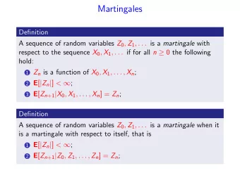
Martingale Let be a sequence of random variables { X t } t ≥ 0 Let be a sequence of -algebras such that { ℱ t } t ≥ 0 σ filtration ℱ 0 ⊆ ℱ 1 ⊆ ℱ 2 ⋯

Martingale Let be a sequence of random variables { X t } t ≥ 0 Let be a sequence of -algebras such that { ℱ t } t ≥ 0 σ filtration ℱ 0 ⊆ ℱ 1 ⊆ ℱ 2 ⋯ A martingale is a sequence of pairs s.t. { X t , ℱ t } t ≥ 0 • for all is -measurable t ≥ 0, X t ℱ t • for all , t ≥ 0 E [ X t +1 ∣ ℱ t ] = X t

Stopping Time

Stopping Time The stopping time is a random variable τ ∈ ℕ ∪ { ∞ } such that is -measurable for all [ τ ≤ t ] ℱ t t

Stopping Time The stopping time is a random variable τ ∈ ℕ ∪ { ∞ } such that is -measurable for all [ τ ≤ t ] ℱ t t “whether to stop can be determined by looking at the outcomes seen so far”

Stopping Time The stopping time is a random variable τ ∈ ℕ ∪ { ∞ } such that is -measurable for all [ τ ≤ t ] ℱ t t “whether to stop can be determined by looking at the outcomes seen so far” • The first time a gambler wins five games in a row • The last time a gambler wins five games in a row

A basic property of a martingale is { X t , ℱ t } t ≥ 0 for any E [ X t ] = E [ X 0 ] t ≥ 0

A basic property of a martingale is { X t , ℱ t } t ≥ 0 for any E [ X t ] = E [ X 0 ] t ≥ 0 Proof. , ∀ t ≥ 1 E [ X t ] = E [ E [ X t ∣ ℱ t − 1 ]] = E [ X t − 1 ]

A basic property of a martingale is { X t , ℱ t } t ≥ 0 for any E [ X t ] = E [ X 0 ] t ≥ 0 Proof. , ∀ t ≥ 1 E [ X t ] = E [ E [ X t ∣ ℱ t − 1 ]] = E [ X t − 1 ] Does hold for a (randomized) E [ X τ ] = E [ X 0 ] stopping time ? τ

A basic property of a martingale is { X t , ℱ t } t ≥ 0 for any E [ X t ] = E [ X 0 ] t ≥ 0 Proof. , ∀ t ≥ 1 E [ X t ] = E [ E [ X t ∣ ℱ t − 1 ]] = E [ X t − 1 ] Does hold for a (randomized) E [ X τ ] = E [ X 0 ] stopping time ? τ Not true in general. Assume is the first time a τ gambler wins $100

Optional Stopping Theorem

Optional Stopping Theorem For a stopping time , holds if τ E [ X τ ] = E [ X 0 ]

Optional Stopping Theorem For a stopping time , holds if τ E [ X τ ] = E [ X 0 ] • Pr[ τ < ∞ ] = 1 • E [ | X τ | ] < ∞ • t →∞ E [ X t ⋅ 1 [ τ > t ] ] = 0 lim

The following conditions are stronger, but easier to verify

The following conditions are stronger, but easier to verify 1. There is a fixed such that a.s. τ ≤ n n 2. and there is a fixed such that Pr[ τ < ∞ ] = 1 M for all | X t | ≤ M t ≤ τ 3. and there is a fixed such that E [ τ ] < ∞ c for all t < τ | X t +1 − X t | ≤ c

The following conditions are stronger, but easier to verify 1. There is a fixed such that a.s. τ ≤ n n 2. and there is a fixed such that Pr[ τ < ∞ ] = 1 M for all | X t | ≤ M t ≤ τ 3. and there is a fixed such that E [ τ ] < ∞ c for all t < τ | X t +1 − X t | ≤ c OST applies when at least one of above holds

Proof of the Optional Stopping Theorem

Applications of OST

Random Walk in 1-D

Random Walk in 1-D t ∑ Let u.a.r. and Z t ∈ { − 1, + 1} X t = Z i i =1

Random Walk in 1-D t ∑ Let u.a.r. and Z t ∈ { − 1, + 1} X t = Z i i =1 The random walk stops when it hits or − a < 0 b > 0

Random Walk in 1-D t ∑ Let u.a.r. and Z t ∈ { − 1, + 1} X t = Z i i =1 The random walk stops when it hits or − a < 0 b > 0 Let be the time it stops. is a stopping time τ τ

Random Walk in 1-D t ∑ Let u.a.r. and Z t ∈ { − 1, + 1} X t = Z i i =1 The random walk stops when it hits or − a < 0 b > 0 Let be the time it stops. is a stopping time τ τ What is ? E [ τ ]

The random walk stops when one of two ends is arrived

The random walk stops when one of two ends is arrived We first determine , the probability that the walk p a ends at , using OST − a

The random walk stops when one of two ends is arrived We first determine , the probability that the walk p a ends at , using OST − a

The random walk stops when one of two ends is arrived We first determine , the probability that the walk p a ends at , using OST − a E [ X τ ] = p a ( − a ) + (1 − p a ) b = E [ X 0 ] = 0

The random walk stops when one of two ends is arrived We first determine , the probability that the walk p a ends at , using OST − a E [ X τ ] = p a ( − a ) + (1 − p a ) b = E [ X 0 ] = 0 b ⟹ p a = a + b

Now define a random variable Y t = X 2 t − t

Now define a random variable Y t = X 2 t − t Claim. is a martingale { Y t } t ≥ 0

Now define a random variable Y t = X 2 t − t Claim. is a martingale { Y t } t ≥ 0 E [ Y t +1 ∣ ℱ t ] = E [( X t + Z t +1 ) 2 − ( t + 1) ∣ ℱ t ] = E [ X 2 t + 2 Z t +1 X t − t ∣ ℱ t ] = X 2 t − t = Y t

satisfies the condition for Y τ OST, so

satisfies the condition for Y τ OST, so E [ Y τ ] = E [ X 2 τ ] − E [ τ ] = E [ Y 0 ] = 0

satisfies the condition for Y τ OST, so E [ Y τ ] = E [ X 2 τ ] − E [ τ ] = E [ Y 0 ] = 0 On the other hand, we have

satisfies the condition for Y τ OST, so E [ Y τ ] = E [ X 2 τ ] − E [ τ ] = E [ Y 0 ] = 0 On the other hand, we have τ ] = p a ⋅ a 2 + (1 − p a ) ⋅ b 2 = ab E [ X 2

satisfies the condition for Y τ OST, so E [ Y τ ] = E [ X 2 τ ] − E [ τ ] = E [ Y 0 ] = 0 On the other hand, we have τ ] = p a ⋅ a 2 + (1 − p a ) ⋅ b 2 = ab E [ X 2 This implies E [ τ ] = ab

Wald’s Equation

Wald’s Equation E [ X i ] N ∑ Recall in Week two, we consider the sum i where are independent with mean and is a { X i } N μ random variable

Wald’s Equation E [ X i ] N ∑ Recall in Week two, we consider the sum i where are independent with mean and is a { X i } N μ random variable

Wald’s Equation E [ X i ] N ∑ Recall in Week two, we consider the sum i where are independent with mean and is a { X i } N μ random variable We are now ready to prove the general case!

t ∑ Assume is finite and let E [ N ] Y t = ( X i − μ ) i =1

t ∑ Assume is finite and let E [ N ] Y t = ( X i − μ ) i =1 is a martingale and the stopping time satisfies { Y t } N the conditions for OST

t ∑ Assume is finite and let E [ N ] Y t = ( X i − μ ) i =1 is a martingale and the stopping time satisfies { Y t } N the conditions for OST E [ Y N ] = E [ ( X i − μ ) ] = E [ X i ] − E [ μ ] N N N ∑ ∑ ∑ i =1 i =1 i =1 = E [ X i ] − E [ N ] ⋅ μ = 0 N ∑ i =1

Waiting Time for Patterns

Waiting Time for Patterns Fix a pattern “00110” P =

Waiting Time for Patterns Fix a pattern “00110” P = How many fair coins one needs to toss to see P for the first time (in expectation)?

Waiting Time for Patterns Fix a pattern “00110” P = How many fair coins one needs to toss to see P for the first time (in expectation)? The number can be calculated using OST

Waiting Time for Patterns Fix a pattern “00110” P = How many fair coins one needs to toss to see P for the first time (in expectation)? The number can be calculated using OST Shuo-Yen Robert Li ( 李碩彥 )

Let the pattern P = p 1 p 2 … p k

Let the pattern P = p 1 p 2 … p k We draw a random string B = b 1 b 2 b 3 …

Let the pattern P = p 1 p 2 … p k We draw a random string B = b 1 b 2 b 3 … Imagine for each , there is a gambler j ≥ 1 G j

Let the pattern P = p 1 p 2 … p k We draw a random string B = b 1 b 2 b 3 … Imagine for each , there is a gambler j ≥ 1 G j At time , bets for “ ”. If he wins, he $1 b j = p 1 j G j bets for “ ”, … $2 b j +1 = p 2

Let the pattern P = p 1 p 2 … p k We draw a random string B = b 1 b 2 b 3 … Imagine for each , there is a gambler j ≥ 1 G j At time , bets for “ ”. If he wins, he $1 b j = p 1 j G j bets for “ ”, … $2 b j +1 = p 2 He keeps doubling the money until he loses

The money of is a martingale (w.r.t. ) G j B

The money of is a martingale (w.r.t. ) G j B Let be the money of all gamblers at time X t t

The money of is a martingale (w.r.t. ) G j B Let be the money of all gamblers at time X t t is also a martingale { X t } t ≥ 1

The money of is a martingale (w.r.t. ) G j B Let be the money of all gamblers at time X t t is also a martingale { X t } t ≥ 1 Let be the first time that we meet in P B τ