Stochastic Processes MATH5835, P. Del Moral UNSW, School of - PowerPoint PPT Presentation

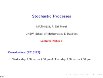
Stochastic Processes MATH5835, P. Del Moral UNSW, School of Mathematics & Statistics Lectures Notes, No. 5 Consultations (RC 5112): Wednesday 3.30 pm � 4.30 pm & Thursday 3.30 pm � 4.30 pm 1/34

Reminder + Information References in the slides ◮ Material for research projects � Moodle ( Stochastic Processes and Applications ∋ variety of applications) ◮ Important results ⊂ Assessment/Final exam = LOGO = 2/34

Citations of the day 3/34

Citations of the day Since the mathematicians have invaded the theory of relativity, I do not understand it myself anymore. 3/34

Citations of the day Since the mathematicians have invaded the theory of relativity, I do not understand it myself anymore. It should be possible to explain the laws of physics to a barmaid. – Albert Einstein (1879-1955) 3/34

Mixture of 3 subjects 1. A complement on martingales 2. A brief reminder on dynamical systems 3. Intro to continuous time stochastic calculus ◮ Brownian motion ◮ Ito(-Doeblin) formula ◮ The heat equation 4/34

Mixture of 3 subjects 1. A complement on martingales 2. A brief reminder on dynamical systems 3. Intro to continuous time stochastic calculus ◮ Brownian motion ◮ Ito(-Doeblin) formula ◮ The heat equation Central/fundamental subjects in stochastic process theory!!!! 4/34

Mixture of 3 subjects 1. A complement on martingales 2. A brief reminder on dynamical systems 3. Intro to continuous time stochastic calculus ◮ Brownian motion ◮ Ito(-Doeblin) formula ◮ The heat equation Central/fundamental subjects in stochastic process theory!!!! ↑ attention 4/34

Mixture of 3 subjects 1. A complement on martingales 2. A brief reminder on dynamical systems 3. Intro to continuous time stochastic calculus ◮ Brownian motion ◮ Ito(-Doeblin) formula ◮ The heat equation Central/fundamental subjects in stochastic process theory!!!! ↑ attention ⊕ ↑ consultation times 4/34

Mixture of 3 subjects 1. A complement on martingales 2. A brief reminder on dynamical systems 3. Intro to continuous time stochastic calculus ◮ Brownian motion ◮ Ito(-Doeblin) formula ◮ The heat equation Central/fundamental subjects in stochastic process theory!!!! ↑ attention ⊕ ↑ consultation times ⊕ ↑ questions 4/34

Mixture of 3 subjects 1. A complement on martingales 2. A brief reminder on dynamical systems 3. Intro to continuous time stochastic calculus ◮ Brownian motion ◮ Ito(-Doeblin) formula ◮ The heat equation Central/fundamental subjects in stochastic process theory!!!! ↑ attention ⊕ ↑ consultation times ⊕ ↑ questions ⇒ ↓ speed 4/34

Designing martingales ϕ n ( ǫ 0 , . . . , ǫ n ) ∈ S (colors, tails/heads, R d ,. . . ) �→ f ( X n ) ∈ R d =1 X n = The natural filtration of information: F n = σ ( ǫ p , 0 ≤ p ≤ n ) = ↑ information ∼ random process 5/34

Designing martingales ϕ n ( ǫ 0 , . . . , ǫ n ) ∈ S (colors, tails/heads, R d ,. . . ) �→ f ( X n ) ∈ R d =1 X n = The natural filtration of information: F n = σ ( ǫ p , 0 ≤ p ≤ n ) = ↑ information ∼ random process Predictable and martingale parts of ∆ f ( X n ) = f ( X n ) − f ( X n − 1 ) 5/34

Designing martingales ϕ n ( ǫ 0 , . . . , ǫ n ) ∈ S (colors, tails/heads, R d ,. . . ) �→ f ( X n ) ∈ R d =1 X n = The natural filtration of information: F n = σ ( ǫ p , 0 ≤ p ≤ n ) = ↑ information ∼ random process Predictable and martingale parts of ∆ f ( X n ) = f ( X n ) − f ( X n − 1 ) ∆ A n ( f ) := E (∆ f ( X n ) | F n − 1 ) = predictable increment 5/34

Designing martingales ϕ n ( ǫ 0 , . . . , ǫ n ) ∈ S (colors, tails/heads, R d ,. . . ) �→ f ( X n ) ∈ R d =1 X n = The natural filtration of information: F n = σ ( ǫ p , 0 ≤ p ≤ n ) = ↑ information ∼ random process Predictable and martingale parts of ∆ f ( X n ) = f ( X n ) − f ( X n − 1 ) ∆ A n ( f ) := E (∆ f ( X n ) | F n − 1 ) = predictable increment ∆ f ( X n ) − E (∆ f ( X n ) | F n − 1 ) = martingale increment ∆ M n ( f ) := 5/34

Designing martingales ϕ n ( ǫ 0 , . . . , ǫ n ) ∈ S (colors, tails/heads, R d ,. . . ) �→ f ( X n ) ∈ R d =1 X n = The natural filtration of information: F n = σ ( ǫ p , 0 ≤ p ≤ n ) = ↑ information ∼ random process Predictable and martingale parts of ∆ f ( X n ) = f ( X n ) − f ( X n − 1 ) ∆ A n ( f ) := E (∆ f ( X n ) | F n − 1 ) = predictable increment ∆ f ( X n ) − E (∆ f ( X n ) | F n − 1 ) = martingale increment ∆ M n ( f ) := Martingale decomposition f ( X n ) = f ( X 0 ) � � + E (∆ f ( X p ) | F p − 1 ) + [∆ f ( X p ) − E (∆ f ( X p ) | F p − 1 )] 1 ≤ p ≤ n 1 ≤ p ≤ n � �� � � �� � Predictable part Martingale part 5/34

An example = The simple Random walk ∆ X n := X n − X n − 1 = ǫ n i.i.d. ǫ n = +1 / − 1 proba 1 / 2 f ( x ) = x & F n = σ ( ǫ p , p ≤ n ) info on the game at time n ∆ A n ( f ) := E (∆ X n | F n − 1 ) = 0 = predictable increment 6/34

An example = The simple Random walk ∆ X n := X n − X n − 1 = ǫ n i.i.d. ǫ n = +1 / − 1 proba 1 / 2 f ( x ) = x & F n = σ ( ǫ p , p ≤ n ) info on the game at time n ∆ A n ( f ) := E (∆ X n | F n − 1 ) = 0 = predictable increment ∆ M n ( f ) := ∆ X n − E (∆ X n | F n − 1 ) = ǫ n = martingale increment f ( x ) = x 3 ( exo ) 6/34

An example = The simple Random walk ∆ X n := X n − X n − 1 = ǫ n i.i.d. ǫ n = +1 / − 1 proba 1 / 2 f ( x ) = x & F n = σ ( ǫ p , p ≤ n ) info on the game at time n ∆ A n ( f ) := E (∆ X n | F n − 1 ) = 0 = predictable increment ∆ M n ( f ) := ∆ X n − E (∆ X n | F n − 1 ) = ǫ n = martingale increment f ( x ) = x 3 ( exo ) ( X n − 1 + ǫ n ) 3 − X 3 X 3 n − X 3 n − 1 = 3 X n − 1 + (3 X 2 = n − 1 + 1) ǫ n n − 1 6/34

An example = The simple Random walk ∆ X n := X n − X n − 1 = ǫ n i.i.d. ǫ n = +1 / − 1 proba 1 / 2 f ( x ) = x & F n = σ ( ǫ p , p ≤ n ) info on the game at time n ∆ A n ( f ) := E (∆ X n | F n − 1 ) = 0 = predictable increment ∆ M n ( f ) := ∆ X n − E (∆ X n | F n − 1 ) = ǫ n = martingale increment f ( x ) = x 3 ( exo ) ( X n − 1 + ǫ n ) 3 − X 3 X 3 n − X 3 n − 1 = 3 X n − 1 + (3 X 2 = n − 1 + 1) ǫ n n − 1 ⇓ � � X 3 n − X 3 ∆ A n ( f ) := n − 1 | F n − 1 = 3 X n − 1 = predictable increment E 6/34

An example = The simple Random walk ∆ X n := X n − X n − 1 = ǫ n i.i.d. ǫ n = +1 / − 1 proba 1 / 2 f ( x ) = x & F n = σ ( ǫ p , p ≤ n ) info on the game at time n ∆ A n ( f ) := E (∆ X n | F n − 1 ) = 0 = predictable increment ∆ M n ( f ) := ∆ X n − E (∆ X n | F n − 1 ) = ǫ n = martingale increment f ( x ) = x 3 ( exo ) ( X n − 1 + ǫ n ) 3 − X 3 X 3 n − X 3 n − 1 = 3 X n − 1 + (3 X 2 = n − 1 + 1) ǫ n n − 1 ⇓ � � X 3 n − X 3 ∆ A n ( f ) := n − 1 | F n − 1 = 3 X n − 1 = predictable increment E (3 X 2 ∆ M n ( f ) := n − 1 + 1) ǫ n = martingale increment 6/34

The martingale 2 [with M 0 = 0] � M 2 (∆ M 2 ) p (∆ M 2 ) p = M 2 p − M 2 = with n p − 1 1 ≤ p ≤ n 7/34

The martingale 2 [with M 0 = 0] � M 2 (∆ M 2 ) p (∆ M 2 ) p = M 2 p − M 2 = with n p − 1 1 ≤ p ≤ n � � � � � � �� ( ∆M 2 ) p | F p − 1 (∆ M 2 ) p − E ( ∆M 2 ) p | F p − 1 = + E 1 ≤ p ≤ n 1 ≤ p ≤ n � �� � = martingale (exo 1) 7/34

The martingale 2 [with M 0 = 0] � M 2 (∆ M 2 ) p (∆ M 2 ) p = M 2 p − M 2 = with n p − 1 1 ≤ p ≤ n � � � � � � �� ( ∆M 2 ) p | F p − 1 (∆ M 2 ) p − E ( ∆M 2 ) p | F p − 1 = + E 1 ≤ p ≤ n 1 ≤ p ≤ n � �� � = martingale (exo 1) � � � � (∆ M 2 ) p | F p − 1 M 2 p − M 2 = p − 1 | F p − 1 E E � � ( M p − M p − 1 ) 2 | F p − 1 = E (exo 2) 7/34

The martingale 2 [with M 0 = 0] � M 2 (∆ M 2 ) p (∆ M 2 ) p = M 2 p − M 2 = with n p − 1 1 ≤ p ≤ n � � � � � � �� ( ∆M 2 ) p | F p − 1 (∆ M 2 ) p − E ( ∆M 2 ) p | F p − 1 = + E 1 ≤ p ≤ n 1 ≤ p ≤ n � �� � = martingale (exo 1) � � � � (∆ M 2 ) p | F p − 1 M 2 p − M 2 = p − 1 | F p − 1 E E � � ( M p − M p − 1 ) 2 | F p − 1 = E (exo 2) Predictable quadratic variation = angle bracket � � (∆ M p ) 2 | F p − 1 � M 2 n = � M � n + Martingale with � M � n := E 1 ≤ p ≤ n 7/34

An example = The simple Random walk M n = M n − 1 + ǫ n i.i.d. ǫ n = +1 / − 1 proba 1 / 2 ⇓ ( M n − 1 + ǫ n ) 2 − M 2 M 2 n − M 2 = n − 1 n − 1 2 M n − 1 ǫ n + ǫ 2 = n = 2 M n − 1 ǫ n + 1 ⇓ � � ( M n − M n − 1 ) 2 | F n − 1 � � M 2 n − M 2 n − 1 | F n − 1 = E = 1 E ⇓ � M 2 n = � M � n + Martingale with � M � n := 1 = n 1 ≤ p ≤ n 8/34

A brief reminder on dynamical systems . X t = b ( X t ) 9/34

A brief reminder on dynamical systems . X t = b ( X t ) ⇐ ⇒ dX t = b ( X t ) dt Key properties: 1. Smooth differentiable trajectories. 2. Fully predictable when we know the initial condition. 3. Well adapted to standard differential calculus. 9/34

� Leibnitz ”long s ” = . X t = b ( X t ) 10/34

� Leibnitz ”long s ” = . ⇐ ⇒ X t = b ( X t ) dX t = b ( X t ) dt 10/34