Algorithms Theory Algorithms Theory 10 10 Greedy Algorithms G d - PowerPoint PPT Presentation

Algorithms Theory Algorithms Theory 10 10 – Greedy Algorithms G d Al ith Dr. Alexander Souza Winter term 11/12

Greedy algorithms 1 1. Introductory remarks Introductory remarks 2. Basic examples: • The coin-changing problem • The traveling salesman problem 3. The activity-selection problem 2 Winter term 11/12

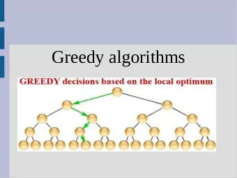
Greedy algorithms for optimization problems y g p p In each step make the choice that p looks best at the moment! Depending on the problem, the outcome can be: 1. The computed solution is always optimal. 2 The computed solution may not be optimal but it 2. The computed solution may not be optimal, but it never differs much from the optimum. 3. The computed solution can be arbitrarily bad. 3 Winter term 11/12

Basic examples: The coin-changing problem Denominations of euro coins and banknotes (in €): Denominations of euro coins and banknotes (in €): 500, 200, 100, 50, 20, 10, 5, 2, 1 Observation Any amount in € can be paid using coins and banknotes of these denominations denominations. Goal Pay an amount n using the fewest number of coins and banknotes possible. 4 Winter term 11/12

Greedy algorithm Greedy algorithm Repeatedly choose the maximum number of coins or banknotes of the largest feasible denomination until the desired sum n is obtained. Example: n = 487 Example: n 487 500 200 100 50 20 10 5 2 1 5 Winter term 11/12

The coin-changing problem: formal description g g p p Denominations of coins: n 1 n 2 Denominations of coins: n 1 , n 2 , ..., n k n k n 1 > n 2 > ... > n k , and n k = 1. Greedy algorithm: 1. w = n 2. for i = 1 to k do 2 f 1 t k d i # coins of denomination n i is m i = ⎣ w / n i ⎦ w = w - m i n i w w m i n i Any amount can be paid! 6 Winter term 11/12

Country ‘Absurdia’ Three denominations: n 3 = 1, n 2 > 1 arbitrary, n 1 = 2 n 2 + 1 Example: 41, 20, 1 Amount to pay: n = 3 n 2 (e.g. n = 60 ) Optimal method of payment: Optimal method of payment: Greedy method: 7 Winter term 11/12

The traveling salesman problem (TSP) Given: n cities, costs c(i,j) to travel from city i to city j Goal: Find a cheapest round-trip route that visits each city exactly once and then returns to the starting city. Formally: Find a permutation p of {1, 2, ..., n } , such that c( p(1), p(2) ) + ••• + c( p(n-1), p(n) ) + c( p(n), p(1) ) ( p( ) p( ) ) ( p( ) p( ) ) ( p( ) p( ) ) is minimzed. 8 Winter term 11/12

The traveling salesman problem (TSP) A greedy algorithm for solving the TSP A greedy algorithm for solving the TSP Starting from city 1, each time go to the nearest city not visited yet. Once all cities have been visited, return to the starting city 1. 9 Winter term 11/12

The traveling salesman problem (TSP) Example Example c( i, i+ 1 ) = 1 , for i = 1, ..., n - 1 c( n, 1 ) = M (for some large number M ) c(i,j) = 2 , otherwise O ti Optimal tour: l t 1 2 3 n – 2 n – 1 n 1 2 3 n 2 n 1 n Solution of the greedy algorithm: 1 1 2 3 n 2 n 1 n 2 3 n – 2 n – 1 n 10 Winter term 11/12

The activity-selection problem Given: A set S A set S = {a 1 ,...,a n } of n activities that wish to use a resource, e.g. a lecture hall. a } of n activities that wish to use a resource e g a lecture hall {a activity a i : start time s i , finish time f i Activities a i and a j are compatible if [ s i f i ) ∩ [ s j f j ) = ∅ [ s i , f i ) ∩ [ s j , f j ) ∅ Goal: S Select a maximum-size subset of mutually compatible activities. f Assumption: p Activities are sorted in non-decreasing order of finish time: f 1 ≤ f 2 ≤ f 3 ≤ ... ≤ f n 11 Winter term 11/12

Greedy strategy for solving the activity-selection problem: Always choose the activity with the earliest finish time Always choose the activity with the earliest finish time that is compatible with all previously selected activities! In particular, the activity chosen first is the one with the earliest finish time. Theorem The greedy strategy for selecting activities yields The greedy strategy for selecting activities yields an optimal solution to the activity-selection problem. 12 Winter term 11/12

The activity-selection problem 2 s i f i 1 3 1 1 4 4 1 3 5 4 1 0 6 5 5 1 4 5 7 6 3 8 1 4 5 5 9 9 7 1 4 6 10 8 8 8 11 11 1 1 4 4 8 12 9 1 4 8 2 13 10 10 12 14 1 4 8 11 1 1 4 4 8 8 1 4 8 11 13 Winter term 11/12 0 1 2 3 4 5 6 7 8 9 10 11 12 13 14

Activity-selection Algorithm Greedy-Activity-Selector Input: Input: n activities represented by intervals [ s f ) 1 ≤ i ≤ n where f ≤ f n activities represented by intervals [ s i , f i ), 1 ≤ i ≤ n , where f i ≤ f i+1 1 Output: a maximum-size set of mutually compatible activities 1 A = { a } 1 A 1 = { a 1 } 2 last = 1 /* last indexes the activity added most recently */ 3 for i = 2 to n do 4 4 if s i < f last if f then A i = A i-1 5 6 else /* s i ≥ f last */ 7 A i = A i-1 ∪ { a i } 8 last = i 9 return A n Running time: O ( n ) 14 Winter term 11/12

Optimality of the greedy algorithm Theorem Theorem The greedy algorithm yields an optimal solution. Proof Show that for all 1 ≤ i ≤ n the following holds: There exists an optimal solution A* with A* ∩ { a 1 ,...., a i } = A i i = 1: i = 1: Let A* ⊆ { a 1 ,...., a n } be some optimal solution, A* = { a i1 ,...., a ik } A* = a i1 a i3 a ik a i2 i2 a 1 15 Winter term 11/12

Optimality of the greedy algorithm i - 1 → i: Let A* ⊆ {a 1 ,...,a n } be some optimal solution with A* ∩ {a 1 ,...,a i-1 } = A i-1 . Consider R Consider R = A* \ A i-1 . A* \ A Observation: R is an optimal solution to the problem of finding a maximum-size set of activities in {a i ,...,a n } that are compatible with all activities in A i-1 . ti iti i } th t tibl ith ll ti iti i { A 16 Winter term 11/12

Optimality of the greedy algorithm Case 1: s i < f last f last A A i-1 = a last a i s i a i is not compatible with A i-1 a i is not contained in A* A* ∩ {a 1 ,...,a i } = A i-1 = A i 17 Winter term 11/12

Optimality of the greedy algorithm Case 2: s i ≥ f last f last A i-1 = a last s i a i a i is compatible with A i-1 There is: R ⊆ {a i ,...,a n } R = b 1 b 2 b 3 b l a i B* = A i-1 ∪ (R \ {b 1 }) ∪ {a i } is optimal B* ∩ {a 1 ,...,a i } = A i-1 ∪ {a i } = A i { 1 i } { i } i 1 i 18 Winter term 11/12

Greedy algorithms Greedy-choice property: Greedy choice property: A globally optimal solution can be attained by a series of locally optimal (greedy) choices. Optimal substructure property: An optimal solution to the problem contains optimal solutions to its An optimal solution to the problem contains optimal solutions to its subproblems. � After making a locally optimal choice a new problem, analogous to the original one, arises. 19 Winter term 11/12