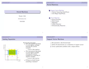
Support Vector Machine and Kernel Methods Jiayu Zhou 1 Department of - PowerPoint PPT Presentation

Support Vector Machine and Kernel Methods Jiayu Zhou 1 Department of Computer Science and Engineering Michigan State University East Lansing, MI USA February 26, 2017 Jiayu Zhou CSE 847 Machine Learning 1 / 50

Which Separator Do You Pick? Jiayu Zhou CSE 847 Machine Learning 2 / 50

Robustness to Noisy Data Being robust to noise (measurement error) is good (remember regularization). Jiayu Zhou CSE 847 Machine Learning 3 / 50

Thicker Cushion Means More Robustness We call such hyperplanes fat Jiayu Zhou CSE 847 Machine Learning 4 / 50

Two Crucial Questions 1 Can we efficiently find the fattest separating hyperplane? 2 Is a fatter hyperplane better than a thin one? Jiayu Zhou CSE 847 Machine Learning 5 / 50

Pulling Out the Bias After Before x ∈ R d ; b ∈ R , w ∈ R d x ∈ { 1 } × R d ; w ∈ R d +1         x 1 w 1 1 w 0 . . x 1 w 1  .   .  x =  ; w =     . .        x =  ; w = . .  .   .  x d w d . .    x d w d bias b signal = w T x signal = w T x + b Jiayu Zhou CSE 847 Machine Learning 6 / 50

Separating The Data Hyperplane h = ( b, w ) h separates the data means: y n ( w T x n + b ) > 0 By rescaling the weights and bias, n =1 ,...,N y n ( w T x n + b ) = 1 min Jiayu Zhou CSE 847 Machine Learning 7 / 50

Distance to the Hyperplane w is normal to the hyperplane (why?) w T ( x 2 − x 1 ) = w T x 2 − w T x 1 = − b + b = 0 Scalar projection: a T b = ∥ a ∥∥ b ∥ cos( a , b ) ⇒ a T b / ∥ b ∥ = ∥ a ∥ cos( a , b ) let x ⊥ be the orthogonal projection of x to h , distance to hyperplane is given by projection of x − x ⊥ to w (why?) 1 ∥ w ∥ · | w T x − w T x ⊥ | dist ( x , h ) = 1 ∥ w ∥ · | w T x + b | = Jiayu Zhou CSE 847 Machine Learning 8 / 50

Fatness of a Separating Hyperplane 1 1 1 ∥ w ∥ · | w T x + b | = ∥ w ∥ · | y n ( w T x + b ) | = ∥ w ∥ · y n ( w T x + b ) dist ( x , h ) = Fatness = Distance to the closest point Fatness = min n dist ( x n , h ) 1 n y n ( w T x + b ) = ∥ w ∥ min 1 = ∥ w ∥ Jiayu Zhou CSE 847 Machine Learning 9 / 50

Maximizing the Margin Formal definition of margin: 1 margin: γ ( h ) = ∥ w ∥ NOTE: Bias b does not appear in the margin. Objective maximizing margin: 1 2 w T w min b, w n =1 ,...,N y n ( w T x n + b ) = 1 subject to: min An equivalent objective: 1 2 w T w min b, w subject to: y n ( w T x n + b ) ≥ 1 for n = 1 , . . . , N Jiayu Zhou CSE 847 Machine Learning 10 / 50

Example - Our Toy Data Set 1 2 w T w min b, w subject to: y n ( w T x n + b ) ≥ 1 for n = 1 , . . . , N Training Data:     0 0 − 1 2 2 − 1     X =  , y =     2 0 +1    3 0 +1 What is the margin? Jiayu Zhou CSE 847 Machine Learning 11 / 50

Example - Our Toy Data Set 1 2 w T w min b, w subject to: y n ( w T x n + b ) ≥ 1 for n = 1 , . . . , N      (1) : − b ≥ 1  0 0 − 1     (2) : − (2 w 1 + 2 w 2 + b ) ≥ 1 2 2 − 1     X =  , y = ⇒     2 0 +1    (3) : 2 w 1 + b ≥ 1    3 0 +1   (4) : 3 w 1 + b ≥ 1 { (1) + (3) → w 1 ≥ 1 → w 2 ≤ − 1 ⇒ 1 2 w T w = 1 2( w 2 1 + w 2 2 ) ≥ 1 (2) + (3) Thus: w 1 = 1 , w 2 = − 1 , b = − 1 Jiayu Zhou CSE 847 Machine Learning 12 / 50

Example - Our Toy Data Set   0 0 2 2   Given data X =   2 0   3 0 Optimal solution [ w 1 = 1 ] w ∗ = , b ∗ = − 1 w 2 = − 1 Optimal hyperplane g ( x ) = sign ( x 1 − x 2 − 1) margin: For data points (1), (2) and 1 1 ∥ w ∥ = 2 ≈ 0 . 707 n w ∗ + b ∗ ) = 1 √ (3) y n ( x T Support Vectors Jiayu Zhou CSE 847 Machine Learning 13 / 50

Solver: Quadratic Programming 1 2 u T Q u + p T u min u ∈ R q subject to: A u ≥ c u ∗ ← QP ( Q, p , A, c ) ( Q = 0 is linear programming.) http://cvxopt.org/examples/tutorial/qp.html Jiayu Zhou CSE 847 Machine Learning 14 / 50

Maximum Margin Hyperplane is QP 1 1 2 w T w 2 u T Q u + p T u min min b, w u ∈ R q subject to: y n ( w T x n + b ) ≥ 1 , ∀ n subject to: A u ≥ c [ b ] [ b ] ∈ R d +1 ⇒ 1 [ 0 T ] [ 0 T ] 0 0 2 w T w = [ b, w T ] = u T u = d d u w T I d I d w 0 d 0 d [ 0 T ] 0 Q = d , p = 0 d +1 I d 0 d y 1 x T y 1 1     1 . . . y n ( w T x n + b ) ≥ 1 = [ y n , y n x T n ] u ≥ 1 ⇒ . .  u ≥ .     . . .    y N x T y N 1 N y 1 x T  y 1   1  1 . . . A = . .  , c = .     . . .    y N x T y N 1 N Jiayu Zhou CSE 847 Machine Learning 15 / 50

Back To Our Example Exercise:      (1) : − b ≥ 1  0 0 − 1     2 2 − 1 (2) : − (2 w 1 + 2 w 2 + b ) ≥ 1     X =  , y =     2 0 +1    (3) : 2 w 1 + b ≥ 1    3 0 +1   (4) : 3 w 1 + b ≥ 1 Show the corresponding Q, p , A, c .     − 1 0 0 1     0 0 0 0 − 1 − 2 − 2 1      , p =  , A = Q = 0 1 0 0  , c =       1 2 0 1    0 0 1 0 1 3 0 1 Use your QP-solver to give u ∗ = [ b ∗ , w ∗ 2 ] T = [ − 1 , 1 , − 1] 1 , w ∗ Jiayu Zhou CSE 847 Machine Learning 16 / 50

Primal QP algorithm for linear-SVM 1 Let p = 0 d +1 be the ( d + 1) -vector of zeros and c = 1 N the N -vector of ones. Construct matrices Q and A , where   − y 1 x T y 1 1 − [ 0 ] 0 T . .  . .  d A =  , Q = . .  I d 0 d − y N x T y N N − [ b ∗ ] = u ∗ ← QP ( Q, p , A, c ) . 2 Return w ∗ 3 The final hypothesis is g ( x ) = sign ( x T w ∗ + b ∗ ) . Jiayu Zhou CSE 847 Machine Learning 17 / 50

Link to Regularization min E in ( w ) w subject to: w T w ≤ C optimal hyperplane regularization w T w minimize E in w T w ≤ C subject to E in = 0 Jiayu Zhou CSE 847 Machine Learning 18 / 50

How to Handle Non-Separable Data? (a) Tolerate noisy data points: soft-margin SVM. (b) Inherent nonlinear boundary: non-linear transformation. Jiayu Zhou CSE 847 Machine Learning 19 / 50

Non-Linear Transformation Φ 1 ( x ) = ( x 1 , x 2 ) Φ 2 ( x ) = ( x 1 , x 2 , x 2 1 , x 1 x 2 , x 2 2 ) Φ 3 ( x ) = ( x 1 , x 2 , x 2 1 , x 1 x 2 , x 2 2 , x 3 1 , x 2 1 x 2 , x 1 x 2 2 , x 3 2 ) Jiayu Zhou CSE 847 Machine Learning 20 / 50

Non-Linear Transformation Using the nonlinear transform with the optimal hyperplane using a transform Φ : R d → R ˜ d : z n = Φ ( x n ) w ∗ , ˜ b ∗ ): Solve the hard-margin SVM in the Z -space ( ˜ 1 w T ˜ min 2 ˜ w ˜ b, ˜ w w T z n + ˜ subject to: y n ( ˜ b ) ≥ 1 , ∀ n Final hypothesis: w ∗ T Φ ( x ) + ˜ b ∗ ) g ( x ) = sign ( ˜ Jiayu Zhou CSE 847 Machine Learning 21 / 50

SVM and non-linear transformation The margin is shaded in yellow, and the support vectors are boxed. For Φ 2 , ˜ d 2 = 5 and for Φ 3 , ˜ d 3 = 9 d 2 is nearly double ˜ ˜ d 3 , yet the resulting SVM separator is not severely overfitting with Φ 3 (regularization?). Jiayu Zhou CSE 847 Machine Learning 22 / 50

Support Vector Machine Summary A very powerful, easy to use linear model which comes with automatic regularization. Fully exploit SVM: Kernel potential robustness to overfitting even after transforming to a much higher dimension How about infinite dimensional transforms? Kernel Trick Jiayu Zhou CSE 847 Machine Learning 23 / 50

SVM Dual: Formulation Primal and dual in optimization. The dual view of SVM enables us to exploit the kernel trick. In the primal SVM problem we solve w ∈ R d , b , while in the dual problem we solve α ∈ R N N N N α n − 1 ∑ ∑ ∑ α n α m y n y m x T max n x m 2 α ∈ R N n =1 m =1 n =1 N ∑ subject to y n α n = 0 , α n ≥ 0 , ∀ n n =1 which is also a QP problem. Jiayu Zhou CSE 847 Machine Learning 24 / 50

SVM Dual: Prediction We can obtain the primal solution: N ∑ w ∗ = y n α ∗ n x n n =1 where for support vectors α n > 0 The optimal hypothesis: g ( x ) = sign ( w ∗ T x + b ∗ ) ( N ) ∑ y n α ∗ n x T n x + b ∗ = sign n =1    ∑ y n α ∗ n x T n x + b ∗ = sign  α ∗ n > 0 Jiayu Zhou CSE 847 Machine Learning 25 / 50

Dual SVM: Summary N N N α n − 1 ∑ ∑ ∑ α n α m y n y m x T max n x m 2 α ∈ R N n =1 m =1 n =1 N ∑ subject to y n α n = 0 , α n ≥ 0 , ∀ n n =1 N ∑ w ∗ = y n α ∗ n x n n =1 Jiayu Zhou CSE 847 Machine Learning 26 / 50

Common SVM Basis Functions z k = polynomial terms of x k of degree 1 to q z k = radial basis function of x k z k ( j ) = φ j ( x k ) = exp( −| x k − c j | 2 /σ 2 ) z k = sigmoid functions of x k Jiayu Zhou CSE 847 Machine Learning 27 / 50