Kernel Interpolation for Scalable Structured Gaussian Processes - PowerPoint PPT Presentation

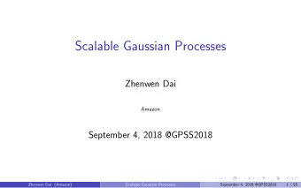
Kernel Interpolation for Scalable Structured Gaussian Processes (KISS-GP) Andrew Gordon Wilson Postdoctoral Research Fellow www.cs.cmu.edu/~andrewgw Carnegie Mellon University Joint work with Hannes Nickisch ICML Lille, France 7 July, 2015 1 / 13

Scalable and Accurate Gaussian Processes ◮ Gaussian processes (GPs) are exactly the types of models we want to apply to big data: flexible function approximators, capable of using the information in large datasets to learn intricate structure through covariance kernels. ◮ However, GPs require O ( n 3 ) computations and O ( n 2 ) storage. ◮ We present a near-exact, O ( n ) , general purpose Gaussian process framework. ◮ This framework i) provides a new unifying perspective of scalable GP approaches, ii) can be used to make predictions with GPs on massive datasets, and iii) enables large-scale kernel learning. ◮ Code is available: http://www.cs.cmu.edu/~andrewgw/pattern 2 / 13

Gaussian process review Definition A Gaussian process (GP) is a collection of random variables, any finite number of which have a joint Gaussian distribution. Nonparametric Regression Model ◮ Prior: f ( x ) ∼ GP ( m ( x ) , k ( x , x ′ )) , meaning ( f ( x 1 ) , . . . , f ( x N )) ∼ N ( µ , K ) , with µ i = m ( x i ) and K ij = cov ( f ( x i ) , f ( x j )) = k ( x i , x j ) . GP posterior GP prior Likelihood � �� � � �� � � �� � p ( f ( x ) |D ) ∝ p ( D| f ( x )) p ( f ( x )) Samples from GP Prior Samples from GP Posterior 4 4 3 3 2 2 Output, f(x) Output, f(x) 1 1 0 0 −1 −1 −2 −2 −3 −3 −4 −4 −10 −5 0 5 10 −10 −5 0 5 10 Input, x Input, x 3 / 13

Inference and Learning 1. Learning: Optimize marginal likelihood, complexity penalty model fit � �� � � �� � − 1 1 2 log | K θ + σ 2 I | − N 2 y T ( K θ + σ 2 I ) − 1 y − log p ( y | θ , X ) = 2 log ( 2 π ) , with respect to kernel hyperparameters θ . The marginal likelihood provides a powerful mechanism for kernel learning . 2. Inference: Conditioned on kernel hyperparameters θ , form the predictive distribution for test inputs X ∗ : f ∗ | X ∗ , X , y , θ ∼ N (¯ f ∗ , cov ( f ∗ )) , ¯ f ∗ = K θ ( X ∗ , X )[ K θ ( X , X ) + σ 2 I ] − 1 y , cov ( f ∗ ) = K θ ( X ∗ , X ∗ ) − K θ ( X ∗ , X )[ K θ ( X , X ) + σ 2 I ] − 1 K θ ( X , X ∗ ) . ( K θ + σ 2 I ) − 1 y and log | K θ + σ 2 I | naively require O ( n 3 ) computations, O ( n 2 ) storage. 4 / 13

Scalable Gaussian Processes Structure Exploiting Approaches Exploit existing structure in K to efficiently solve linear systems and log determinants. ◮ Examples: Kronecker Structure, K = K 1 ⊗ K 2 ⊗ · · · ⊗ K P . Toeplitz Structure: K ij = K i + 1 , j + 1 . ◮ Extremely efficient and accurate, but require severe grid assumptions. Inducing Point Approaches Introduce m inducing points , U = { u i } m i = 1 , and approximate K X , X ≈ K X , U K − 1 U , U K U , X . ◮ SoR, DTC, FITC, Big Data GP ◮ General purpose, but requires m ≪ n for efficiency, which degrades accuracy and prohibits expressive kernel learning. Can we create a new framework that combines the benefits of each approach? 5 / 13

A New Unifying Framework ◮ Recall m × m n × n n × m m × n ���� � �� � ���� ���� K − 1 K SoR ( X , X ) = K X , U K U , X (1) U , U ◮ Complexity is O ( m 2 n + m 3 ) . ◮ It is tempting to place inducing points on a grid to create structure in K U , U , but this only helps with the m 3 term, not the more critical m 2 n term coming from K X , U . ◮ Can we approximate K X , U from K U , U ? 6 / 13

Kernel Interpolation For example, if we want to approximate k ( x , u ) , we could form k ( x , u ) ≈ wk ( u a , u ) + ( 1 − w ) k ( u b , u ) , (2) where u a ≤ x ≤ u b . More generally, we form K X , U ≈ WK U , U , (3) where W is an n × m sparse matrix of interpolation weights. For local linear interpolation W has only c = 2 non-zero entries per row. For local cubic interpolation, c = 4. Substituting K X , U ≈ WK U , U into the inducing point approximation, U , U K U , U W T = WK U , U W T = K SKI . K X , X ≈ K X , U K − 1 U , U K U , X ≈ WK U , U K − 1 7 / 13

Kernel Interpolation n × m m × m ���� ���� K U , U W T K SKI = W (4) ◮ MVMs with W cost O ( n ) computations and storage. ◮ Toeplitz K U , U : MVMs cost O ( m log m ) . ◮ Kronecker structure in K U , U : MVMs cost O ( Pm 1 + 1 / P ) . Conclusions ◮ MVMs with K SKI cost O ( n ) computations and storage! ◮ We can therefore solve K − 1 SKI y using linear conjugate gradients in j ≪ n iterations, for GP inference. ◮ Even if the inputs X do not have any structure, we can naturally create structure in the latent variables U which can be exploited for greatly accelerated inference and learning. ◮ We can use m ≫ n inducing points! (Accuracy and kernel learning) 8 / 13

New Unifying Framework It turns out that all inducing methods perform global GP interpolation on a user-specified kernel! ◮ The predictive mean of a noise-free, zero mean GP ( σ = 0 , µ ( x ) ≡ 0) is linear in two ways: on the one hand, as a w X ( x ∗ ) = K − 1 X , X K X , x ∗ weighted sum of the observations y , and on the other hand as an α = K − 1 X , X y weighted sum of training-test cross-covariances K X , x ∗ : ¯ f ∗ = y T w X ( x ∗ ) = α T K X , x ∗ . (5) ◮ If we are to perform a noise free zero-mean GP regression on the kernel itself, such that we have data D = ( u i , k ( u i , x )) m i = 1 , then we recover the inducing kernel ˜ k SoR ( x , z ) = K U , x K − 1 U , U K U , z as the predictive mean of the GP at test point x ∗ = z ! 9 / 13

Local versus Global Kernel Interpolation 1 1 k k k(U,u) k(U,u) Global Local 0.75 0.75 Covariance Covariance k SoR (x,u) k SKI (x,u) 0.5 0.5 0.25 0.25 0 0 0 2.5 5 7.5 10 0 2.5 5 7.5 10 x x (c) Global Kernel Interpolation (d) Local Kernel Interpolation Figure: Global vs. local kernel interpolation. Triangle markers denote the inducing points used for interpolating k ( x , u ) from k ( U , u ) . Here u = 0, U = { 0 , 1 , . . . , 10 } , and x = 3 . 4. a) All conventional inducing point methods, such as SoR or FITC, perform global GP regression on K U , u (a vector of covariances between all inducing points U and the point u ), at test point x ∗ = x , to form an approximate ˜ k , e.g., k SoR ( x , u ) = K x , U K − 1 U , U K U , u , for any desired x and u . b) SKI can perform local kernel interpolation on K U , u to form the approximation k SKI ( x , u ) = w T x K U , u . 10 / 13

Kernel Matrix Reconstruction −5 x 10 1 1 0.1 equi−linear 200 0.8 200 0.8 200 15 0.08 kmeans−linear equi−GP Error 0.06 400 0.6 400 0.6 400 equi−cubic 10 0.04 600 0.4 600 0.4 600 5 0.02 800 0.2 800 0.2 800 0 10 15 20 25 1000 1000 1000 200 400 600 800 1000 200 400 600 800 1000 200 400 600 800 1000 m (a) K true (b) K SKI ( m = 40 ) (c) | K true − K SKI, 40 | (d) Interpolation Strategies −8 −8 x 10 x 10 −4 10 14 SKI (linear) 4 12 200 200 SoR −6 10 10 FITC 3 Error 400 400 8 SKI (cubic) 2 600 600 6 −8 10 4 800 1 800 2 −10 10 0 0.1 0.2 0.3 0.4 1000 1000 200 400 600 800 1000 200 400 600 800 1000 Runtime (s) (e) | K true − K SKI, 150 | (f) | K true − K SoR, 150 | (g) Error vs Runtime 11 / 13

Kernel Learning 1 True 0.8 FITC Correlation Correlation SKI 0.5 0.6 0.4 0 0.2 0 −0.5 −0.2 0 0.5 1 0 0.5 1 τ τ Figure: Kernel Learning. A product of two kernels (shown in green) was used to sample 10 , 000 datapoints from a GP. From this data, we performed kernel learning using SKI (cubic) and FITC, with the results shown in blue and red, respectively. All kernels are a function of τ = x − x ′ and are scaled by k ( 0 ) . 12 / 13

Natural Sound Modelling 3 10 0.2 Runtime (s) 0.1 Intensity 2 10 FITC 0 SKI (cubic) 1 10 −0.1 −0.2 0 10 0 1 2 3 2500 3000 3500 4000 4500 5000 Time (s) m (a) Natural Sound (b) Runtime vs m 0.8 0.7 0.6 SMAE 0.5 0.4 0.3 0.2 0 1 2 3 10 10 10 10 Runtime (s) (c) Error vs Runtime Figure: Natural Sound Modelling 13 / 13