Style Surface Illustration with B- Spline Models James Mower - - PowerPoint PPT Presentation

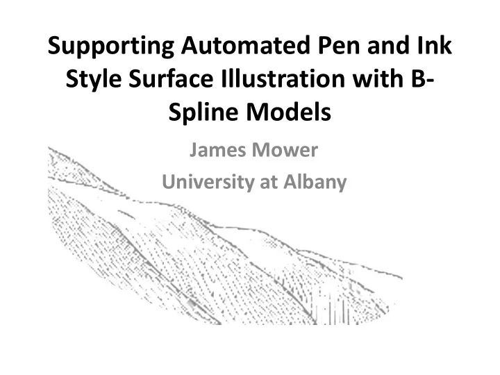
Supporting Automated Pen and Ink Style Surface Illustration with B- Spline Models

James Mower University at Albany

• Demonstrated in Tuscan landscape paintings

by da Vinci

• Extended to

woodcuts in the 16th century by Murer and

• thers

Perspective Landscape Rendering

Section of Map of Zurich, Murer, 1566 Study of a Tuscan Landscape, Da Vinci, ca. 1473

Geomorphological Illustrators

Automating Pen and Ink Illustration

• Apply a non-photorealistic rendering (NPR)

approach

• Use an “economy of lines”

– Markosian and others, 1997

• Depict the essential form of an object using a

minimal number of strokes

Linework

• Landscape features

are represented with 2 types of linework

– Silhouettes

• Boundaries between

visible and invisible surfaces

– Form Lines

• Surface trends

W.M. Davis

• More samples, less interpolation
• TIN
• Polyhedron
• Interpolated values lie on plane
• Fewer samples, more interpolation
• “Global” polynomial functions of order p
• Polynomial patches of order p
• Interpolated values evaluate to degree p-1 surface

Representing Elevation

But Which Is Best?

• Manual pen and ink style landscape

illustrations usually depict low noise surfaces

• Dense sampling models have lots of noise
• Some NPR techniques are sensitive to noise

– Can generate numerous junk silhouettes

• Bezier surface models supress noise and are

good candidates for NPR support

Surface Noise and Silhouettes

Bezier Surface Models

• A Bezier surface is described by control points
• Its order in u and v equals the number of

control points along the respective axes

• Each control point is associated with a basis

function

• The basis function determines the control

point’s influence on the surface at position u,v

A Bezier Surface

A degree 3 by degree 3 Bezier Surface

Generated from a Java applet created by David Little, Department of Mathematics, Penn State

A Problem with Bezier Surfaces

• Evaluation times increase exponentially with

the number of control points

• Computations on large numbers of control

points can lead to numerical overflow

• Solution—B-Spline surfaces

– A patchwork of low order Bezier surfaces – Stitched together at their edges with continuous joins

B-Spline Surface Model

• Composed of local ‘basis’ functions that only

contribute within a given ‘knot span’

• The continuity at the joins is determined by:

– The degree of the basis functions in u and v – The number of duplicate knot values at the join

• This project uses degree 3 basis functions with

2 times differentiability at the joins

A B-Spline Surface

10 degree 3 by degree 3 patches are stitched together with 2 times differentiability at patch borders

Surface Tessellation

• Polynomial surfaces are rendered as a set of

planar facets (a tessellation)

• The facets should cover about

the same screen space, regardless of their position in the world

• The OpenGL B-spline rendering functions

enforce this criterion

Gray Shaded B-Spline Surface

Rendering this surface in emissive white makes it a useful surface mask for silhouette and form line rendering

Surface Processing Environment

• OpenGL

– NURBS (non-uniform, rational B-spline) package

• CGAL

– Computational Geometry and Algorithms Library – Triangulation facilities – Useful geometric modeling operations and primitives

• Written in C++ for MS Windows

Extracting Silhouettes

Silhouettes and a Masking Surface

Defining Form Lines

• A form line shows a surface trend
• Form lines can be defined globally or locally
• This project defines a form line segment as a

line of steepest descent from one vertex to an adjacent neighbor

– Form lines are visual composites of locally generated segments

The Form Line Model

The weighted illumination and slope components control shading for a surface facet

Using Drainage Accumulation Models

• Lines of steepest descent are assembled into a

stream network

• Each branch of

the network has a stream order

• Segments can

be displayed or hidden by order

Simulated Effect

Form Line Example

Rendering Parameters

• Illumination azimuth and altitude
• Position and attitude of the viewpoint
• Variable form line width with slope and

illumination angles

• Form line display by stream order
• Adjustable weighting of all parameters

Varying Illumination Azimuth

72 images, illumination azimuth rotating through 360 degrees at 5 degrees per image West Temple feature, Zion National Park

Level of Detail Varies with the Viewpoint Position

100 still images on an 8 km flight path

When Less is More

• This W.M. Davis image uses very few strokes
• The following slide

shows how a landscape can be rendered with fewer strokes

A Low Relief Environment

• This is from a coastal scene in Labrador

– DEM provided by Rudy Slingerlands at Penn State

• Not as minimal as Davis, but getting there…

Performance Issues and a New Approach

• Building silhouette and drainage models with

CGAL from NURBS models is very slow

– The Utah images take 5 to 10 minutes per frame

• New OpenGL versions allow tessellation

control with shader programs

• Shader programs run on the GPU and can be

very fast

Preliminary GPU Results

• Now doing B-spline modeling on the GPU
• Silhouettes are interpreted as borders

between rendered pixels generated from non 3D-contiguous parent triangles

• Speeds are approaching animation time scale

Thanks for Coming!

• A couple recent papers are at

http://www.albany.edu/faculty/jmower/geog/ publications/

• Any questions?