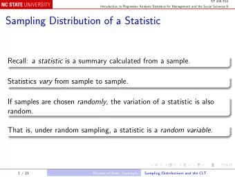
Statistics 430/514 Introduction to Regression Analysis/ Statistics - - PowerPoint PPT Presentation

ST 430/514 Introduction to Regression Analysis/Statistics for Management and the Social Sciences II

Statistics 430/514

Introduction to Regression Analysis/ Statistics for Management and the Social Sciences II

Instructor: Peter Bloomfield Course home page:

http://www.stat.ncsu.edu/people/bloomfield/courses/ST430-514/

1 / 19

ST 430/514 Introduction to Regression Analysis/Statistics for Management and the Social Sciences II

Review of Statistical Concepts

Definition Statistics is the science of data. This involves collecting, classifying, summarizing, organizing, analyzing, and interpreting data. Data are collected by observing specified quantities, called variables, related to entities called experimental units.

2 / 19 Review of Basic Concepts Statistics and Data

ST 430/514 Introduction to Regression Analysis/Statistics for Management and the Social Sciences II

Example In a public opinion poll, people (the experimental units) are queried about their: age (a quantatitive variable); gender (a qualitative variable, here with 2 levels); party affiliation (another qualitative variable, with more than 2 levels);

• pinion of Hillary Clinton (another qualitative variable)
• pinion of Marco Rubio (yet another qualitative variable)

3 / 19 Review of Basic Concepts Statistics and Data

ST 430/514 Introduction to Regression Analysis/Statistics for Management and the Social Sciences II

Population and Sample

Population We are usually interested in the characteristics of a population, but

• bserving all experimental units in the population is infeasible.

For example, we might be interested in the opinions of all registered voters in North Carolina. That defines the population.

4 / 19 Review of Basic Concepts Populations and Samples

ST 430/514 Introduction to Regression Analysis/Statistics for Management and the Social Sciences II

Sample So we observe a sample from that population, and make (statistical) inferences about the population based on the sample data. For example, we might contact 2,000 people by dialing random telephone numbers, reaching 1,150 registered voters. We might infer that their opinions are representative of the whole state. So if the sample shows 57% have a favorable opinion of Clinton, 36% unfavorable, and 7% not sure, we infer that those are the most likely figures statewide.

5 / 19 Review of Basic Concepts Populations and Samples

ST 430/514 Introduction to Regression Analysis/Statistics for Management and the Social Sciences II

Naturally, our inference is highly unlikely to be exactly correct. But a large, well collected sample is likely to be closer than a smaller

• r less well collected sample.

A measure of reliability is a statement about degree of uncertainty of a statistical inference. For instance, the margin of error for the opinion poll is around ±3%. That is, the chance that any population percentage differs from the sample percentage by more than 3% is small (≤ .05).

6 / 19 Review of Basic Concepts Populations and Samples

ST 430/514 Introduction to Regression Analysis/Statistics for Management and the Social Sciences II

Summarizing qualitative data

A qualitative variable like voting intention is usually summarized as a percentage, as above. It may be displayed graphically as a bar graph (or histogram), or in a pie chart. In R

Clinton <- c(favorable = 57, unfavorable = 36, notsure = 7) barplot(Clinton) pie(Clinton)

7 / 19 Review of Basic Concepts Describing Qualitative Data

ST 430/514 Introduction to Regression Analysis/Statistics for Management and the Social Sciences II

Rubio <- c(favorable = 35, unfavorable = 27, notsure = 38) par(mfrow = c(1, 2)) pie(Clinton) title("Clinton") pie(Rubio) title("Rubio")

8 / 19 Review of Basic Concepts Describing Qualitative Data

ST 430/514 Introduction to Regression Analysis/Statistics for Management and the Social Sciences II

Summarizing quantitative data

M&S example EPA’s fuel consumption measurements for 100 cars (same model and year).

epagas <- read.table("Text/Exercises&Examples/EPAGAS.txt", header = TRUE)

A graphical summary

hist(epagas$MPG) # to match Figure 1.6: hist(epagas$MPG, breaks = 30:45, right = FALSE)

9 / 19 Review of Basic Concepts Describing Quantitative Data

ST 430/514 Introduction to Regression Analysis/Statistics for Management and the Social Sciences II

A semi-graphical display Stem and leaf:

stem(epagas$MPG) # to match Figure 1.5: stem(epagas$MPG, scale = 2)

Notes A summary describes the data, but suppresses some details. The second stem-and-leaf plot displays the data, but is not a summary, because no details are omitted. We cannot recover the original data from the first plot, so it is a

• summary. Similarly, if the data had more decimal places, the

stem-and-leaf plot would show only the most significant digit in the leaf, so then it would be a summary.

10 / 19 Review of Basic Concepts Describing Quantitative Data

ST 430/514 Introduction to Regression Analysis/Statistics for Management and the Social Sciences II

Numerical summaries:

The mean of data y1, y2, . . . , yn: ¯ y = 1 n

n

• i=1

yi. In R

mean(epagas$MPG) # 36.994

The corresponding population quantity is the population mean: µ = E(Y ).

11 / 19 Review of Basic Concepts Describing Quantitative Data

ST 430/514 Introduction to Regression Analysis/Statistics for Management and the Social Sciences II

The variance of data y1, y2, . . . , yn: s2 = 1 n − 1

n

• i=1

(yi − ¯ y)2 . In R

var(epagas$MPG) # 5.846226

The corresponding population quantity is the population variance: σ2 = E

• (Y − µ)2

.

12 / 19 Review of Basic Concepts Describing Quantitative Data

ST 430/514 Introduction to Regression Analysis/Statistics for Management and the Social Sciences II

The units of variance are the square of the units of the data. So for instance the variance of the fuel consumption data is 5.846226 (mpg)2. The standard deviation is the square root of the variance: s = √ s2 σ = √ σ2. In R

sd(epagas$MPG) # 2.417897; we could also use sqrt(var(epagas$MPG))

With units: s = 2.417897 mpg ≈ 2.42 mpg.

13 / 19 Review of Basic Concepts Describing Quantitative Data

ST 430/514 Introduction to Regression Analysis/Statistics for Management and the Social Sciences II

Interpreting the mean and standard deviation

In any data set or population, at least 75% of the data lie within two standard deviations of the mean, by Tchebysheff’s Theorem. If the data are approximately normally distributed, around 95% of the data lie within two standard deviations of the mean.

14 / 19 Review of Basic Concepts Describing Quantitative Data

ST 430/514 Introduction to Regression Analysis/Statistics for Management and the Social Sciences II

Sample Statistic A summary calculated from sample data is a statistic. Population Parameter The corresponding population quantity is a parameter, such as the average fuel consumption for the tested car model, averaged over the entire production. Statistical Inference We usually do not know the value of a parameter, but we use the statistics of a sample to make inferences about it. Sampling Variability Statistics vary from sample to sample.

15 / 19 Review of Basic Concepts Describing Quantitative Data

ST 430/514 Introduction to Regression Analysis/Statistics for Management and the Social Sciences II

The Normal Probability Distribution

The standard normal distribution (µ = 0, σ = 1):

−3 −2 −1 1 2 3 0.0 0.1 0.2 0.3 0.4 x

Standard normal density

16 / 19 Review of Basic Concepts The Normal Probability Distribution

ST 430/514 Introduction to Regression Analysis/Statistics for Management and the Social Sciences II

Normal distributions with (µ = −4, σ = 0.5), (µ = 0, σ = 1.5), and (µ = 3, σ = 1.0):

−6 −4 −2 2 4 6 0.0 0.2 0.4 0.6 0.8 x

Three normal densities

17 / 19 Review of Basic Concepts The Normal Probability Distribution

ST 430/514 Introduction to Regression Analysis/Statistics for Management and the Social Sciences II

Standardizing: if Y has the normal distribution with mean µ and standard deviation σ, then Z = Y − µ σ has mean 0 and standard deviation 1, so it follows the standard normal distribution. One key fact about the standard normal distribution is that P(|Z| ≤ 1.96) = .95, and hence also P(µ − 1.96σ ≤ Y ≤ µ + 1.96σ) = .95

18 / 19 Review of Basic Concepts The Normal Probability Distribution

ST 430/514 Introduction to Regression Analysis/Statistics for Management and the Social Sciences II

For instance, if the fuel consumption Y of a car chosen randomly from a year’s production had the normal distribution with µ = 37 mpg and standard deviation σ = 2.4 mpg, then Z = Y − 37 2.4 follows the standard normal distribution. Then P(|Z| ≤ 1.96) = .95 implies that .95 = P

• Y − 37

2.4

• ≤ 1.96
• = P(37 − 1.96 × 2.4 ≤ Y ≤ 37 + 1.96 × 2.4).

In words, there is a 95% chance that the car’s fuel consumption will be between 32.3 and 41.7 mpg.

19 / 19 Review of Basic Concepts The Normal Probability Distribution