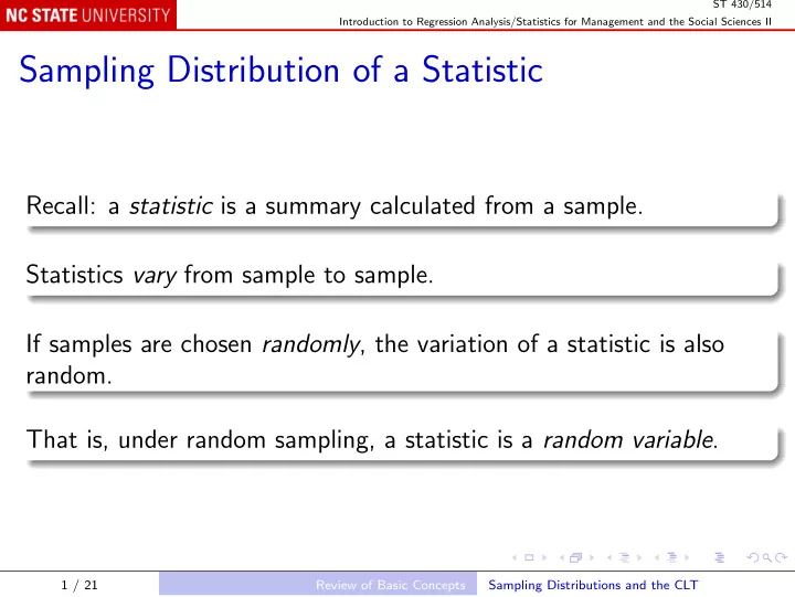
Sampling Distribution of a Statistic Recall: a statistic is a summary - - PowerPoint PPT Presentation

ST 430/514 Introduction to Regression Analysis/Statistics for Management and the Social Sciences II

Sampling Distribution of a Statistic

Recall: a statistic is a summary calculated from a sample. Statistics vary from sample to sample. If samples are chosen randomly, the variation of a statistic is also random. That is, under random sampling, a statistic is a random variable.

1 / 21 Review of Basic Concepts Sampling Distributions and the CLT

ST 430/514 Introduction to Regression Analysis/Statistics for Management and the Social Sciences II

Sampling Distribution Every random variable has a probability distribution, usually represented by either: a probability density function, such as a normal density;

• r a probability mass function, such as the binomial or Poisson

probability functions. In the special case of a statistic, its probability distribution is also called its sampling distribution.

2 / 21 Review of Basic Concepts Sampling Distributions and the CLT

ST 430/514 Introduction to Regression Analysis/Statistics for Management and the Social Sciences II

Fuel Consumption Example For example, suppose we view the 100 fuel consumption values as a population, and draw a random sample of size 25: mean(sample(epagas$MPG, 25)) # 36.944 If we draw more samples, we get a different sample mean each time: mean(sample(epagas$MPG, 25)) # 37.044 mean(sample(epagas$MPG, 25)) # 37.088

3 / 21 Review of Basic Concepts Sampling Distributions and the CLT

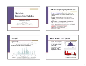
ST 430/514 Introduction to Regression Analysis/Statistics for Management and the Social Sciences II

If we draw many samples, we begin to see the sampling distribution:

sampleMeans = rep(NA, 1000) for (i in 1:length(sampleMeans)) sampleMeans[i] = mean(sample(epagas$MPG, 25)) hist(sampleMeans)

Note that the sample means are: distributed around the population mean of 37 mpg; not as widely dispersed as the original 100 measurements.

4 / 21 Review of Basic Concepts Sampling Distributions and the CLT

ST 430/514 Introduction to Regression Analysis/Statistics for Management and the Social Sciences II

Some Theoretical Results If Y1, Y2, . . . , Yn are randomly sampled from some population with mean µ and standard deviation σ, then the sampling distribution of their mean ¯ Y satisfies: for any n, Mean: E ¯ Y

• = µ ¯

Y = µ,

Standard error of estimate: σ ¯

Y = σ

√n for large n, ¯ Y is approximately normally distributed (Central Limit Theorem).

5 / 21 Review of Basic Concepts Sampling Distributions and the CLT

ST 430/514 Introduction to Regression Analysis/Statistics for Management and the Social Sciences II

Inference About a Parameter: Point Estimation

For example, the population mean, µ A good estimator of µ should have a sampling distribution that is: centered around µ with little dispersion. We often make these ideas specific by using the mean and standard error. Consider the sample mean, ¯ Y : centering: µ ¯

Y = µ; ¯

Y is unbiased; dispersion: σ ¯

Y = σ/√n; ¯

Y has a small standard error of estimate when n is large.

6 / 21 Review of Basic Concepts Point Estimate of a Population Mean

ST 430/514 Introduction to Regression Analysis/Statistics for Management and the Social Sciences II

In fact, when the original data are normally distributed, ¯ Y has the smallest standard error of any unbiased estimator. That is, the sample mean ¯ Y is a Minimum Variance Unbiased Estimator (MVUE). In other cases, ¯ Y is usally a good estimator of µ, but not the best. For data with the uniform distribution, the midrange is better. For data with the double exponential (Laplace) distribution, the sample median is better.

7 / 21 Review of Basic Concepts Point Estimate of a Population Mean

ST 430/514 Introduction to Regression Analysis/Statistics for Management and the Social Sciences II

The sample mean ¯ Y is always the Best Linear Unbiased Estimator (BLUE): For any constants w1, w2, . . . , wn with wi = 1, if W is the estimator W =

n

• i=1

wiYi then W is unbiased: µW =

n

• i=1

wiµ = µ; but the standard error of estimate is σW =

• n
• i=1

w 2

i σ2 ≥ σ

√n = σ ¯

Y .

8 / 21 Review of Basic Concepts Point Estimate of a Population Mean

ST 430/514 Introduction to Regression Analysis/Statistics for Management and the Social Sciences II

Inference About a Parameter: Interval Estimation

Recall that, by the Central Limit Theorem, when n is large, ¯ Y is approximately normally distributed. That is, ¯ Y − µ ¯

Y

σ ¯

Y

= ¯ Y − µ σ/√n approximately follows the standard normal distribution.

9 / 21 Review of Basic Concepts Confidence Interval for a Population Mean

ST 430/514 Introduction to Regression Analysis/Statistics for Management and the Social Sciences II

So the chance that µ − 1.96 σ √n ≤ ¯ Y ≤ µ + 1.96 σ √n is approximately 95%. Equivalently, the chance that ¯ Y − 1.96 σ √n ≤ µ ≤ ¯ Y + 1.96 σ √n is approximately 95%. We say that ¯ Y ± 1.96 σ √n is an approximate 95% confidence interval (CI) for µ.

10 / 21 Review of Basic Concepts Confidence Interval for a Population Mean

ST 430/514 Introduction to Regression Analysis/Statistics for Management and the Social Sciences II

To calculate the end-points of this approximate confidence interval, we need to know the additional parameter σ. Typically σ is unknown, so we cannot use the CI. But we can estimate σ by the sample standard deviation s, and use the alternative confidence interval ¯ Y ± 1.96 s √n. When n is large, the chance that ¯ Y − 1.96 s √n ≤ µ ≤ ¯ Y + 1.96 s √n is still approximately 95%.

11 / 21 Review of Basic Concepts Confidence Interval for a Population Mean

ST 430/514 Introduction to Regression Analysis/Statistics for Management and the Social Sciences II

What if n is not large? In small samples, we can still construct a confidence interval, but it has the correct coverage probability only if the original data are approximately normally distributed. The key is to replace ±1.96, the 2.5% and 97.5% points of the normal distribution, with ±t.025,n−1, the 2.5% and 97.5% points of Student’s t-distribution with (n − 1) degrees of freedom: for normally distributed data, the chance that ¯ Y − t.025,n−1 s √n ≤ µ ≤ ¯ Y + t.025,n−1 s √n is 95%.

12 / 21 Review of Basic Concepts Confidence Interval for a Population Mean

ST 430/514 Introduction to Regression Analysis/Statistics for Management and the Social Sciences II

Tables of the t-distribution show that when n is large, the percent points are very close to those of the normal distribution. So it’s reasonable to use the t-distribution percent points whenever the confidence interval is based on the sample s instead of the population σ. M&S give formulas for a general 100(1 − α)% confidence interval: ¯ Y ± tα/2,n−1 s √n; here α = .05 for a 95% CI; in some situations, α = .01 for a 99% CI is preferred; other values are rarely used.

13 / 21 Review of Basic Concepts Confidence Interval for a Population Mean

ST 430/514 Introduction to Regression Analysis/Statistics for Management and the Social Sciences II

Inference About a Parameter: Testing a Hypothesis

A point estimate is the most likely value of the parameter. A confidence interval is a calibrated range of plausible values. Sometimes we just want to know whether a particular value is plausible. We assess its plausibility by testing statistical hypotheses.

14 / 21 Review of Basic Concepts Testing a Hypothesis About a Mean

ST 430/514 Introduction to Regression Analysis/Statistics for Management and the Social Sciences II

Example: µ0 is an interesting value of the population mean µ. Null hypothesis, H0: µ = µ0 Alternative hypothesis, Ha: µ = µ0. Data are a sample of size n with mean ¯ y and standard deviation s. Basic idea: H0 is implausible if ¯ y is far from µ0.

15 / 21 Review of Basic Concepts Testing a Hypothesis About a Mean

ST 430/514 Introduction to Regression Analysis/Statistics for Management and the Social Sciences II

To be precise: t = |¯ y − µ0| s/√n measures how far ¯ y is from µ0, as a multiple of the standard error of estimate. Basic idea: reject H0 if t is large. To be precise: choose a level of significance α; again often α = .05. Reject H0 if t > tα/2,n−1.

16 / 21 Review of Basic Concepts Testing a Hypothesis About a Mean

ST 430/514 Introduction to Regression Analysis/Statistics for Management and the Social Sciences II

We can show that when H0 is true, that is µ = µ0, and the data are normally distributed, the chance of (incorrectly) rejecting H0 is α. That is, α is the chance of making a Type I error. If a statistician always follows this procedure, true null hypotheses will be rejected only 100α% of the time. So when a null hypothesis is rejected, either it was actually false, or

• ne of these infrequent errors occurred.

Note: We never accept H0, we only fail to reject it.

17 / 21 Review of Basic Concepts Testing a Hypothesis About a Mean

ST 430/514 Introduction to Regression Analysis/Statistics for Management and the Social Sciences II

This is a two-tailed test: we reject H0 if ¯ y is too far from µ0 in either direction. In regression analysis, almost all tests are two-tailed. M&S discuss one-tailed tests, and provide an example. Deciding which hypothesis is H0 and which is Ha may not be easy.

18 / 21 Review of Basic Concepts Testing a Hypothesis About a Mean

ST 430/514 Introduction to Regression Analysis/Statistics for Management and the Social Sciences II

Example: Reading scores Data are changes in reading scores after an experimental reading program, relative to baseline scores. We are interested in whether the program leads to a change, either improvement or degradation, so µ0 = 0: H0 : µ = 0; Ha : µ = 0. n = 8, ¯ y = 4.375, s = 1.685, t = 7.34. We reject H0.

19 / 21 Review of Basic Concepts Testing a Hypothesis About a Mean

ST 430/514 Introduction to Regression Analysis/Statistics for Management and the Social Sciences II

P-value Instead of deciding whether to reject H0, we can weigh the evidence against it. The conventional way to do this is using the P-value, which is: the probability, if H0 were true, that the test statistic is as extreme as observed. In the reading score example, P(|t| ≥ 7.34) = .00016 A small P-value like this is strong evidence against H0.

20 / 21 Review of Basic Concepts Testing a Hypothesis About a Mean

ST 430/514 Introduction to Regression Analysis/Statistics for Management and the Social Sciences II

Other Hypothesis Tests

Some other hypothesis tests are commonly used, and you should be familiar with them. However, some are not particularly useful in regression analysis. Two described in M&S are: Comparing the means of two populations; H0 : µ1 = µ2 versus Ha : µ1 = µ2; Comparing the variances of two populations; H0 : σ2

1 = σ2 2 versus

Ha : σ2

1 = σ2 2.

21 / 21 Review of Basic Concepts Other Hypothesis Tests