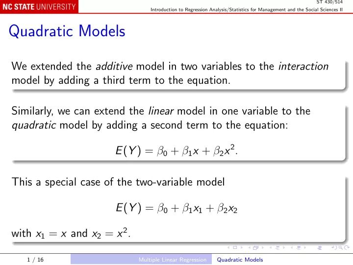
Quadratic Models We extended the additive model in two variables to - PowerPoint PPT Presentation

ST 430/514 Introduction to Regression Analysis/Statistics for Management and the Social Sciences II Quadratic Models We extended the additive model in two variables to the interaction model by adding a third term to the equation. Similarly, we can extend the linear model in one variable to the quadratic model by adding a second term to the equation: E ( Y ) = β 0 + β 1 x + β 2 x 2 . This a special case of the two-variable model E ( Y ) = β 0 + β 1 x 1 + β 2 x 2 with x 1 = x and x 2 = x 2 . 1 / 16 Multiple Linear Regression Quadratic Models

ST 430/514 Introduction to Regression Analysis/Statistics for Management and the Social Sciences II Example: immune system and exercise x = maximal oxygen uptake (VO 2 max, mL / (kg · min)); y = immunoglobulin level (IgG, mg / dL); data for 30 subjects (AEROBIC.txt). Get the data and plot them: aerobic <- read.table("Text/Exercises&Examples/AEROBIC.txt", header = TRUE) plot(aerobic[, c("MAXOXY", "IGG")]) Slight curvature suggests a linear model may not fit. 2 / 16 Multiple Linear Regression Quadratic Models

ST 430/514 Introduction to Regression Analysis/Statistics for Management and the Social Sciences II Check the linear model: plot(lm(IGG ~ MAXOXY, aerobic)) Graph of residuals against fitted values shows definite curvature. Fit and summarize the quadratic model: aerobicLm <- lm(IGG ~ MAXOXY + I(MAXOXY^2), aerobic) summary(aerobicLm) 3 / 16 Multiple Linear Regression Quadratic Models

ST 430/514 Introduction to Regression Analysis/Statistics for Management and the Social Sciences II Output Call: lm(formula = IGG ~ MAXOXY + I(MAXOXY^2), data = aerobic) Residuals: Min 1Q Median 3Q Max -185.375 -82.129 1.047 66.007 227.377 Coefficients: Estimate Std. Error t value Pr(>|t|) (Intercept) -1464.4042 411.4012 -3.560 0.00140 ** MAXOXY 88.3071 16.4735 5.361 1.16e-05 *** I(MAXOXY^2) -0.5362 0.1582 -3.390 0.00217 ** --- Signif. codes: 0 *** 0.001 ** 0.01 * 0.05 . 0.1 1 Residual standard error: 106.4 on 27 degrees of freedom Multiple R-squared: 0.9377, Adjusted R-squared: 0.9331 F-statistic: 203.2 on 2 and 27 DF, p-value: < 2.2e-16 4 / 16 Multiple Linear Regression Quadratic Models

ST 430/514 Introduction to Regression Analysis/Statistics for Management and the Social Sciences II The quadratic term I(MAXOXY^2) is significant, so we reject the null hypothesis that the linear model is acceptable. The quadratic term is negative, which is consistent with the concavity of the curve. The other two t -ratios test irrelevant hypotheses, because the quadratic term is important. Extrapolation: the fitted curve has a maximum at 88 . 3071 MAXOXY = 2 × 0 . 5362 ≈ 82 and declines for higher MAXOXY , which seems unlikely to represent the real relationship. 5 / 16 Multiple Linear Regression Quadratic Models

ST 430/514 Introduction to Regression Analysis/Statistics for Management and the Social Sciences II An alternative analysis The graph of IGG against log(MAXOXY) is more linear: with(aerobic, plot(log(MAXOXY), IGG)) aerobicLm2 <- lm(IGG ~ log(MAXOXY), aerobic) summary(aerobicLm2) with(aerobic, plot(MAXOXY, IGG)) with(aerobic, lines(sort(MAXOXY), fitted(aerobicLm)[order(MAXOXY)], col = "blue")) with(aerobic, lines(sort(MAXOXY), fitted(aerobicLm2)[order(MAXOXY)], col = "red")) The fitted curve continues to increase indefinitely, but with diminishing slope. 6 / 16 Multiple Linear Regression Quadratic Models

ST 430/514 Introduction to Regression Analysis/Statistics for Management and the Social Sciences II Output Call: lm(formula = IGG ~ log(MAXOXY), data = aerobic) Residuals: Min 1Q Median 3Q Max -165.455 -88.651 -2.395 55.756 218.934 Coefficients: Estimate Std. Error t value Pr(>|t|) (Intercept) -4885.71 324.33 -15.06 5.87e-15 *** log(MAXOXY) 1653.38 83.07 19.90 < 2e-16 *** --- Signif. codes: 0 *** 0.001 ** 0.01 * 0.05 . 0.1 1 Residual standard error: 107.6 on 28 degrees of freedom Multiple R-squared: 0.934, Adjusted R-squared: 0.9316 F-statistic: 396.1 on 1 and 28 DF, p-value: < 2.2e-16 7 / 16 Multiple Linear Regression Quadratic Models

ST 430/514 Introduction to Regression Analysis/Statistics for Management and the Social Sciences II More Complex Models Complete second-order model When the first-order model E ( Y ) = β 0 + β 1 x 1 + β 2 x 2 is inadequate, the interaction model E ( Y ) = β 0 + β 1 x 1 + β 2 x 2 + β 3 x 1 x 2 may be better, but sometimes a complete second-order model is needed: E ( Y ) = β 0 + β 1 x 1 + β 2 x 2 + β 3 x 1 x 2 + β 4 x 2 1 + β 5 x 2 2 8 / 16 Multiple Linear Regression More Complex Models

ST 430/514 Introduction to Regression Analysis/Statistics for Management and the Social Sciences II Example: cost of shipping packages Get the data and plot them: express <- read.table("Text/Exercises&Examples/EXPRESS.txt", header = TRUE) pairs(express) Fit the complete second-order model and summarize it: expressLm <- lm(Cost ~ Weight * Distance + I(Weight^2) + I(Distance^2), express) summary(expressLm) plot(expressLm) 9 / 16 Multiple Linear Regression More Complex Models

ST 430/514 Introduction to Regression Analysis/Statistics for Management and the Social Sciences II Output Call: lm(formula = Cost ~ Weight * Distance + I(Weight^2) + I(Distance^2), data = express) Residuals: Min 1Q Median 3Q Max -0.86027 -0.19898 -0.00885 0.16531 0.94396 Coefficients: Estimate Std. Error t value Pr(>|t|) (Intercept) 8.270e-01 7.023e-01 1.178 0.258588 Weight -6.091e-01 1.799e-01 -3.386 0.004436 ** Distance 4.021e-03 7.998e-03 0.503 0.622999 I(Weight^2) 8.975e-02 2.021e-02 4.442 0.000558 *** I(Distance^2) 1.507e-05 2.243e-05 0.672 0.512657 Weight:Distance 7.327e-03 6.374e-04 11.495 1.62e-08 *** --- Signif. codes: 0 *** 0.001 ** 0.01 * 0.05 . 0.1 1 Residual standard error: 0.4428 on 14 degrees of freedom Multiple R-squared: 0.9939, Adjusted R-squared: 0.9918 F-statistic: 458.4 on 5 and 14 DF, p-value: 5.371e-15 10 / 16 Multiple Linear Regression More Complex Models

ST 430/514 Introduction to Regression Analysis/Statistics for Management and the Social Sciences II Qualitative Variables A qualitative variable (or factor ) is one that indicates membership of different categories. E.g., a person’s gender = male or female : a qualitative variable with two levels , indicating membership of one of two categories. E.g., package type = Fragile , Semifragile , or Durable : three levels, corresponding to three categories. 11 / 16 Multiple Linear Regression More Complex Models

ST 430/514 Introduction to Regression Analysis/Statistics for Management and the Social Sciences II We code a qualitative variable using indicator (dummy) variables: Choose one level to use as a base or reference level, say male or Durable . For each other level, create a variable � 1 if this item is in this category x j = 0 otherwise. For gender, there is only one other category, so the only indicator variable is � 1 for a female x = 0 for a male. 12 / 16 Multiple Linear Regression More Complex Models

ST 430/514 Introduction to Regression Analysis/Statistics for Management and the Social Sciences II For packages, there are two other categories, so the indicator variables are � 1 for a Fragile package x Fragile = 0 otherwise, � 1 for a Semifragile package x Semifragile = 0 otherwise, For any item, at most one of the indicator variables is non-zero, indicating a non-base category; if they are all zero, the item belongs to the base category. 13 / 16 Multiple Linear Regression More Complex Models

ST 430/514 Introduction to Regression Analysis/Statistics for Management and the Social Sciences II Example: shipment cost of packages, by type. Get the data and plot them: cargo <- read.table("Text/Exercises&Examples/CARGO.txt", header = TRUE) plot(COST ~ CARGO, cargo) Fit and summarize the model: cargoLm <- lm(COST ~ CARGO, cargo) summary(cargoLm) 14 / 16 Multiple Linear Regression More Complex Models

ST 430/514 Introduction to Regression Analysis/Statistics for Management and the Social Sciences II Output Call: lm(formula = COST ~ CARGO, data = cargo) Residuals: Min 1Q Median 3Q Max -2.20 -1.80 -1.00 1.05 4.24 Coefficients: Estimate Std. Error t value Pr(>|t|) (Intercept) 3.260 1.075 3.032 0.0104 * CARGOFragile 9.740 1.521 6.405 3.38e-05 *** CARGOSemiFrag 5.440 1.521 3.577 0.0038 ** --- Signif. codes: 0 *** 0.001 ** 0.01 * 0.05 . 0.1 1 Residual standard error: 2.404 on 12 degrees of freedom Multiple R-squared: 0.7745, Adjusted R-squared: 0.7369 F-statistic: 20.61 on 2 and 12 DF, p-value: 0.0001315 15 / 16 Multiple Linear Regression More Complex Models

ST 430/514 Introduction to Regression Analysis/Statistics for Management and the Social Sciences II Note that the intercept is the fitted value for CARGOFragile = 0 and CARGOSemiFrag = 0 ; that is, for Durable packages. The coefficients of CARGOFragile and CARGOSemiFrag measure the differences between those categories and Durable . The overall model F -test is the same as the analysis of variance test: cargoAov <- aov(COST ~ CARGO, cargo) summary(cargoAov) Output Df Sum Sq Mean Sq F value Pr(>F) CARGO 2 238.25 119.13 20.61 0.000132 *** Residuals 12 69.37 5.78 --- Signif. codes: 0 *** 0.001 ** 0.01 * 0.05 . 0.1 1 16 / 16 Multiple Linear Regression More Complex Models