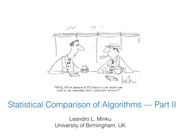
Statistical Comparison of Algorithms Part II Leandro L. Minku - PowerPoint PPT Presentation
Statistical Comparison of Algorithms Part II Leandro L. Minku University of Birmingham, UK Overview Recap of the general idea underlying statistical hypothesis tests. What to compare? Two algorithms on a single problem instance.
<latexit sha1_base64="GW1PktPxj4HaWVW6dkVJYLRBxk=">ACBnicbZDLSgMxFIYz9VbrbdSlCMEiuLHOFEGXRTduKhXsBTpDyaSZNjTJjElGKMOs3Pgqblwo4tZncOfbmLaz0OoPgY/nMPJ+YOYUaUd58sqLCwuLa8UV0tr6xubW/b2TktFicSkiSMWyU6AFGFUkKampFOLAniASPtYHQ5qbfviVQ0Erd6HBOfo4GgIcVIG6tn73uhRDitu8f1apZ6ig4OvHUndTpdZb17LJTcaCf8HNoQxyNXr2p9ePcMKJ0JghpbquE2s/RVJTzEhW8hJFYoRHaEC6BgXiRPnp9IwMHhqnD8NImic0nLo/J1LElRrzwHRypIdqvjYx/6t1Ex2e+ykVcaKJwLNFYcKgjuAkE9inkmDNxgYQltT8FeIhMrlok1zJhODOn/wXWtWKa/jmtFy7yOMogj1wAI6AC85ADVyBmgCDB7AE3gBr9aj9Wy9We+z1oKVz+yCX7I+vgEfIZjn</latexit> <latexit sha1_base64="GW1PktPxj4HaWVW6dkVJYLRBxk=">ACBnicbZDLSgMxFIYz9VbrbdSlCMEiuLHOFEGXRTduKhXsBTpDyaSZNjTJjElGKMOs3Pgqblwo4tZncOfbmLaz0OoPgY/nMPJ+YOYUaUd58sqLCwuLa8UV0tr6xubW/b2TktFicSkiSMWyU6AFGFUkKampFOLAniASPtYHQ5qbfviVQ0Erd6HBOfo4GgIcVIG6tn73uhRDitu8f1apZ6ig4OvHUndTpdZb17LJTcaCf8HNoQxyNXr2p9ePcMKJ0JghpbquE2s/RVJTzEhW8hJFYoRHaEC6BgXiRPnp9IwMHhqnD8NImic0nLo/J1LElRrzwHRypIdqvjYx/6t1Ex2e+ykVcaKJwLNFYcKgjuAkE9inkmDNxgYQltT8FeIhMrlok1zJhODOn/wXWtWKa/jmtFy7yOMogj1wAI6AC85ADVyBmgCDB7AE3gBr9aj9Wy9We+z1oKVz+yCX7I+vgEfIZjn</latexit> <latexit sha1_base64="GW1PktPxj4HaWVW6dkVJYLRBxk=">ACBnicbZDLSgMxFIYz9VbrbdSlCMEiuLHOFEGXRTduKhXsBTpDyaSZNjTJjElGKMOs3Pgqblwo4tZncOfbmLaz0OoPgY/nMPJ+YOYUaUd58sqLCwuLa8UV0tr6xubW/b2TktFicSkiSMWyU6AFGFUkKampFOLAniASPtYHQ5qbfviVQ0Erd6HBOfo4GgIcVIG6tn73uhRDitu8f1apZ6ig4OvHUndTpdZb17LJTcaCf8HNoQxyNXr2p9ePcMKJ0JghpbquE2s/RVJTzEhW8hJFYoRHaEC6BgXiRPnp9IwMHhqnD8NImic0nLo/J1LElRrzwHRypIdqvjYx/6t1Ex2e+ykVcaKJwLNFYcKgjuAkE9inkmDNxgYQltT8FeIhMrlok1zJhODOn/wXWtWKa/jmtFy7yOMogj1wAI6AC85ADVyBmgCDB7AE3gBr9aj9Wy9We+z1oKVz+yCX7I+vgEfIZjn</latexit> <latexit sha1_base64="GW1PktPxj4HaWVW6dkVJYLRBxk=">ACBnicbZDLSgMxFIYz9VbrbdSlCMEiuLHOFEGXRTduKhXsBTpDyaSZNjTJjElGKMOs3Pgqblwo4tZncOfbmLaz0OoPgY/nMPJ+YOYUaUd58sqLCwuLa8UV0tr6xubW/b2TktFicSkiSMWyU6AFGFUkKampFOLAniASPtYHQ5qbfviVQ0Erd6HBOfo4GgIcVIG6tn73uhRDitu8f1apZ6ig4OvHUndTpdZb17LJTcaCf8HNoQxyNXr2p9ePcMKJ0JghpbquE2s/RVJTzEhW8hJFYoRHaEC6BgXiRPnp9IwMHhqnD8NImic0nLo/J1LElRrzwHRypIdqvjYx/6t1Ex2e+ykVcaKJwLNFYcKgjuAkE9inkmDNxgYQltT8FeIhMrlok1zJhODOn/wXWtWKa/jmtFy7yOMogj1wAI6AC85ADVyBmgCDB7AE3gBr9aj9Wy9We+z1oKVz+yCX7I+vgEfIZjn</latexit> General Idea — Z Test for Two Population Means, Variance Known Formulate Hypotheses: • H0: μ 1 = μ 2 —> μ 1 - μ 2 = 0 • H1: μ 1 ≠ μ 2 —> μ 1 - μ 2 ≠ 0 • • Level of significance α = 0.05 (probability of Type I error). M 1 − M 2 Test statistic Z = • √ σ / N Theoretical sampling distribution of the test statistic assuming H0 is • true: normal distribution. But there is still a small chance that H0 was true (Type I error). =1/2 level of significance of 0.05 =1/2 level of 8 significance of 0.05
<latexit sha1_base64="GW1PktPxj4HaWVW6dkVJYLRBxk=">ACBnicbZDLSgMxFIYz9VbrbdSlCMEiuLHOFEGXRTduKhXsBTpDyaSZNjTJjElGKMOs3Pgqblwo4tZncOfbmLaz0OoPgY/nMPJ+YOYUaUd58sqLCwuLa8UV0tr6xubW/b2TktFicSkiSMWyU6AFGFUkKampFOLAniASPtYHQ5qbfviVQ0Erd6HBOfo4GgIcVIG6tn73uhRDitu8f1apZ6ig4OvHUndTpdZb17LJTcaCf8HNoQxyNXr2p9ePcMKJ0JghpbquE2s/RVJTzEhW8hJFYoRHaEC6BgXiRPnp9IwMHhqnD8NImic0nLo/J1LElRrzwHRypIdqvjYx/6t1Ex2e+ykVcaKJwLNFYcKgjuAkE9inkmDNxgYQltT8FeIhMrlok1zJhODOn/wXWtWKa/jmtFy7yOMogj1wAI6AC85ADVyBmgCDB7AE3gBr9aj9Wy9We+z1oKVz+yCX7I+vgEfIZjn</latexit> <latexit sha1_base64="GW1PktPxj4HaWVW6dkVJYLRBxk=">ACBnicbZDLSgMxFIYz9VbrbdSlCMEiuLHOFEGXRTduKhXsBTpDyaSZNjTJjElGKMOs3Pgqblwo4tZncOfbmLaz0OoPgY/nMPJ+YOYUaUd58sqLCwuLa8UV0tr6xubW/b2TktFicSkiSMWyU6AFGFUkKampFOLAniASPtYHQ5qbfviVQ0Erd6HBOfo4GgIcVIG6tn73uhRDitu8f1apZ6ig4OvHUndTpdZb17LJTcaCf8HNoQxyNXr2p9ePcMKJ0JghpbquE2s/RVJTzEhW8hJFYoRHaEC6BgXiRPnp9IwMHhqnD8NImic0nLo/J1LElRrzwHRypIdqvjYx/6t1Ex2e+ykVcaKJwLNFYcKgjuAkE9inkmDNxgYQltT8FeIhMrlok1zJhODOn/wXWtWKa/jmtFy7yOMogj1wAI6AC85ADVyBmgCDB7AE3gBr9aj9Wy9We+z1oKVz+yCX7I+vgEfIZjn</latexit> <latexit sha1_base64="GW1PktPxj4HaWVW6dkVJYLRBxk=">ACBnicbZDLSgMxFIYz9VbrbdSlCMEiuLHOFEGXRTduKhXsBTpDyaSZNjTJjElGKMOs3Pgqblwo4tZncOfbmLaz0OoPgY/nMPJ+YOYUaUd58sqLCwuLa8UV0tr6xubW/b2TktFicSkiSMWyU6AFGFUkKampFOLAniASPtYHQ5qbfviVQ0Erd6HBOfo4GgIcVIG6tn73uhRDitu8f1apZ6ig4OvHUndTpdZb17LJTcaCf8HNoQxyNXr2p9ePcMKJ0JghpbquE2s/RVJTzEhW8hJFYoRHaEC6BgXiRPnp9IwMHhqnD8NImic0nLo/J1LElRrzwHRypIdqvjYx/6t1Ex2e+ykVcaKJwLNFYcKgjuAkE9inkmDNxgYQltT8FeIhMrlok1zJhODOn/wXWtWKa/jmtFy7yOMogj1wAI6AC85ADVyBmgCDB7AE3gBr9aj9Wy9We+z1oKVz+yCX7I+vgEfIZjn</latexit> <latexit sha1_base64="GW1PktPxj4HaWVW6dkVJYLRBxk=">ACBnicbZDLSgMxFIYz9VbrbdSlCMEiuLHOFEGXRTduKhXsBTpDyaSZNjTJjElGKMOs3Pgqblwo4tZncOfbmLaz0OoPgY/nMPJ+YOYUaUd58sqLCwuLa8UV0tr6xubW/b2TktFicSkiSMWyU6AFGFUkKampFOLAniASPtYHQ5qbfviVQ0Erd6HBOfo4GgIcVIG6tn73uhRDitu8f1apZ6ig4OvHUndTpdZb17LJTcaCf8HNoQxyNXr2p9ePcMKJ0JghpbquE2s/RVJTzEhW8hJFYoRHaEC6BgXiRPnp9IwMHhqnD8NImic0nLo/J1LElRrzwHRypIdqvjYx/6t1Ex2e+ykVcaKJwLNFYcKgjuAkE9inkmDNxgYQltT8FeIhMrlok1zJhODOn/wXWtWKa/jmtFy7yOMogj1wAI6AC85ADVyBmgCDB7AE3gBr9aj9Wy9We+z1oKVz+yCX7I+vgEfIZjn</latexit> General Idea — Z Test for Two Population Means, Variance Known Formulate Hypotheses: • H0: μ 1 = μ 2 —> μ 1 - μ 2 = 0 • H1: μ 1 ≠ μ 2 —> μ 1 - μ 2 ≠ 0 • • Level of significance α = 0.05 (probability of Type I error). M 1 − M 2 Test statistic Z = • √ σ / N Theoretical sampling distribution of the test statistic assuming H0 is • true: normal distribution. Critical region is the set of test statistic values that would lead to rejecting H0. =1/2 level of significance of 0.05 =1/2 level of 9 significance of 0.05
<latexit sha1_base64="GW1PktPxj4HaWVW6dkVJYLRBxk=">ACBnicbZDLSgMxFIYz9VbrbdSlCMEiuLHOFEGXRTduKhXsBTpDyaSZNjTJjElGKMOs3Pgqblwo4tZncOfbmLaz0OoPgY/nMPJ+YOYUaUd58sqLCwuLa8UV0tr6xubW/b2TktFicSkiSMWyU6AFGFUkKampFOLAniASPtYHQ5qbfviVQ0Erd6HBOfo4GgIcVIG6tn73uhRDitu8f1apZ6ig4OvHUndTpdZb17LJTcaCf8HNoQxyNXr2p9ePcMKJ0JghpbquE2s/RVJTzEhW8hJFYoRHaEC6BgXiRPnp9IwMHhqnD8NImic0nLo/J1LElRrzwHRypIdqvjYx/6t1Ex2e+ykVcaKJwLNFYcKgjuAkE9inkmDNxgYQltT8FeIhMrlok1zJhODOn/wXWtWKa/jmtFy7yOMogj1wAI6AC85ADVyBmgCDB7AE3gBr9aj9Wy9We+z1oKVz+yCX7I+vgEfIZjn</latexit> <latexit sha1_base64="GW1PktPxj4HaWVW6dkVJYLRBxk=">ACBnicbZDLSgMxFIYz9VbrbdSlCMEiuLHOFEGXRTduKhXsBTpDyaSZNjTJjElGKMOs3Pgqblwo4tZncOfbmLaz0OoPgY/nMPJ+YOYUaUd58sqLCwuLa8UV0tr6xubW/b2TktFicSkiSMWyU6AFGFUkKampFOLAniASPtYHQ5qbfviVQ0Erd6HBOfo4GgIcVIG6tn73uhRDitu8f1apZ6ig4OvHUndTpdZb17LJTcaCf8HNoQxyNXr2p9ePcMKJ0JghpbquE2s/RVJTzEhW8hJFYoRHaEC6BgXiRPnp9IwMHhqnD8NImic0nLo/J1LElRrzwHRypIdqvjYx/6t1Ex2e+ykVcaKJwLNFYcKgjuAkE9inkmDNxgYQltT8FeIhMrlok1zJhODOn/wXWtWKa/jmtFy7yOMogj1wAI6AC85ADVyBmgCDB7AE3gBr9aj9Wy9We+z1oKVz+yCX7I+vgEfIZjn</latexit> <latexit sha1_base64="GW1PktPxj4HaWVW6dkVJYLRBxk=">ACBnicbZDLSgMxFIYz9VbrbdSlCMEiuLHOFEGXRTduKhXsBTpDyaSZNjTJjElGKMOs3Pgqblwo4tZncOfbmLaz0OoPgY/nMPJ+YOYUaUd58sqLCwuLa8UV0tr6xubW/b2TktFicSkiSMWyU6AFGFUkKampFOLAniASPtYHQ5qbfviVQ0Erd6HBOfo4GgIcVIG6tn73uhRDitu8f1apZ6ig4OvHUndTpdZb17LJTcaCf8HNoQxyNXr2p9ePcMKJ0JghpbquE2s/RVJTzEhW8hJFYoRHaEC6BgXiRPnp9IwMHhqnD8NImic0nLo/J1LElRrzwHRypIdqvjYx/6t1Ex2e+ykVcaKJwLNFYcKgjuAkE9inkmDNxgYQltT8FeIhMrlok1zJhODOn/wXWtWKa/jmtFy7yOMogj1wAI6AC85ADVyBmgCDB7AE3gBr9aj9Wy9We+z1oKVz+yCX7I+vgEfIZjn</latexit> <latexit sha1_base64="GW1PktPxj4HaWVW6dkVJYLRBxk=">ACBnicbZDLSgMxFIYz9VbrbdSlCMEiuLHOFEGXRTduKhXsBTpDyaSZNjTJjElGKMOs3Pgqblwo4tZncOfbmLaz0OoPgY/nMPJ+YOYUaUd58sqLCwuLa8UV0tr6xubW/b2TktFicSkiSMWyU6AFGFUkKampFOLAniASPtYHQ5qbfviVQ0Erd6HBOfo4GgIcVIG6tn73uhRDitu8f1apZ6ig4OvHUndTpdZb17LJTcaCf8HNoQxyNXr2p9ePcMKJ0JghpbquE2s/RVJTzEhW8hJFYoRHaEC6BgXiRPnp9IwMHhqnD8NImic0nLo/J1LElRrzwHRypIdqvjYx/6t1Ex2e+ykVcaKJwLNFYcKgjuAkE9inkmDNxgYQltT8FeIhMrlok1zJhODOn/wXWtWKa/jmtFy7yOMogj1wAI6AC85ADVyBmgCDB7AE3gBr9aj9Wy9We+z1oKVz+yCX7I+vgEfIZjn</latexit> General Idea — Z Test for Two Population Means, Variance Known Formulate Hypotheses: • H0: μ 1 = μ 2 —> μ 1 - μ 2 = 0 • H1: μ 1 ≠ μ 2 —> μ 1 - μ 2 ≠ 0 • • Level of significance α = 0.05 (probability of Type I error). M 1 − M 2 Test statistic Z = • √ σ / N Theoretical sampling distribution of the test statistic assuming H0 is • true: normal distribution. Critical values are the “boundary” values of the critical region. 10
<latexit sha1_base64="GW1PktPxj4HaWVW6dkVJYLRBxk=">ACBnicbZDLSgMxFIYz9VbrbdSlCMEiuLHOFEGXRTduKhXsBTpDyaSZNjTJjElGKMOs3Pgqblwo4tZncOfbmLaz0OoPgY/nMPJ+YOYUaUd58sqLCwuLa8UV0tr6xubW/b2TktFicSkiSMWyU6AFGFUkKampFOLAniASPtYHQ5qbfviVQ0Erd6HBOfo4GgIcVIG6tn73uhRDitu8f1apZ6ig4OvHUndTpdZb17LJTcaCf8HNoQxyNXr2p9ePcMKJ0JghpbquE2s/RVJTzEhW8hJFYoRHaEC6BgXiRPnp9IwMHhqnD8NImic0nLo/J1LElRrzwHRypIdqvjYx/6t1Ex2e+ykVcaKJwLNFYcKgjuAkE9inkmDNxgYQltT8FeIhMrlok1zJhODOn/wXWtWKa/jmtFy7yOMogj1wAI6AC85ADVyBmgCDB7AE3gBr9aj9Wy9We+z1oKVz+yCX7I+vgEfIZjn</latexit> <latexit sha1_base64="GW1PktPxj4HaWVW6dkVJYLRBxk=">ACBnicbZDLSgMxFIYz9VbrbdSlCMEiuLHOFEGXRTduKhXsBTpDyaSZNjTJjElGKMOs3Pgqblwo4tZncOfbmLaz0OoPgY/nMPJ+YOYUaUd58sqLCwuLa8UV0tr6xubW/b2TktFicSkiSMWyU6AFGFUkKampFOLAniASPtYHQ5qbfviVQ0Erd6HBOfo4GgIcVIG6tn73uhRDitu8f1apZ6ig4OvHUndTpdZb17LJTcaCf8HNoQxyNXr2p9ePcMKJ0JghpbquE2s/RVJTzEhW8hJFYoRHaEC6BgXiRPnp9IwMHhqnD8NImic0nLo/J1LElRrzwHRypIdqvjYx/6t1Ex2e+ykVcaKJwLNFYcKgjuAkE9inkmDNxgYQltT8FeIhMrlok1zJhODOn/wXWtWKa/jmtFy7yOMogj1wAI6AC85ADVyBmgCDB7AE3gBr9aj9Wy9We+z1oKVz+yCX7I+vgEfIZjn</latexit> <latexit sha1_base64="GW1PktPxj4HaWVW6dkVJYLRBxk=">ACBnicbZDLSgMxFIYz9VbrbdSlCMEiuLHOFEGXRTduKhXsBTpDyaSZNjTJjElGKMOs3Pgqblwo4tZncOfbmLaz0OoPgY/nMPJ+YOYUaUd58sqLCwuLa8UV0tr6xubW/b2TktFicSkiSMWyU6AFGFUkKampFOLAniASPtYHQ5qbfviVQ0Erd6HBOfo4GgIcVIG6tn73uhRDitu8f1apZ6ig4OvHUndTpdZb17LJTcaCf8HNoQxyNXr2p9ePcMKJ0JghpbquE2s/RVJTzEhW8hJFYoRHaEC6BgXiRPnp9IwMHhqnD8NImic0nLo/J1LElRrzwHRypIdqvjYx/6t1Ex2e+ykVcaKJwLNFYcKgjuAkE9inkmDNxgYQltT8FeIhMrlok1zJhODOn/wXWtWKa/jmtFy7yOMogj1wAI6AC85ADVyBmgCDB7AE3gBr9aj9Wy9We+z1oKVz+yCX7I+vgEfIZjn</latexit> <latexit sha1_base64="GW1PktPxj4HaWVW6dkVJYLRBxk=">ACBnicbZDLSgMxFIYz9VbrbdSlCMEiuLHOFEGXRTduKhXsBTpDyaSZNjTJjElGKMOs3Pgqblwo4tZncOfbmLaz0OoPgY/nMPJ+YOYUaUd58sqLCwuLa8UV0tr6xubW/b2TktFicSkiSMWyU6AFGFUkKampFOLAniASPtYHQ5qbfviVQ0Erd6HBOfo4GgIcVIG6tn73uhRDitu8f1apZ6ig4OvHUndTpdZb17LJTcaCf8HNoQxyNXr2p9ePcMKJ0JghpbquE2s/RVJTzEhW8hJFYoRHaEC6BgXiRPnp9IwMHhqnD8NImic0nLo/J1LElRrzwHRypIdqvjYx/6t1Ex2e+ykVcaKJwLNFYcKgjuAkE9inkmDNxgYQltT8FeIhMrlok1zJhODOn/wXWtWKa/jmtFy7yOMogj1wAI6AC85ADVyBmgCDB7AE3gBr9aj9Wy9We+z1oKVz+yCX7I+vgEfIZjn</latexit> General Idea — Z Test for Two Population Means, Variance Known Formulate Hypotheses: • H0: μ 1 = μ 2 —> μ 1 - μ 2 = 0 • H1: μ 1 ≠ μ 2 —> μ 1 - μ 2 ≠ 0 • • Level of significance α = 0.05 (probability of Type I error). M 1 − M 2 Test statistic Z = • √ σ / N Theoretical sampling distribution of the test statistic assuming H0 is • true: normal distribution. P-value: probability of observing test • statistic value at least as extreme as the value z, assuming H0, is the AUC of the region starting at z and -z. If p-value ≤ α , reject H0. • Otherwise, do not reject H0 • -z z 11
Terminology • For two tailed test (H0: μ 1 = μ 2, H1: μ 1 ≠ μ 2): • Not rejecting H0: no statistically significant difference has been found between μ 1 and μ 2 at the level of significance of α = 0.05 (p- value of …). • It doesn’t mean that we accept H0, it just means that we have not found enough evidence to reject it. G.K. Kanji. 100 Statistical Tests. Chapter “Introduction to Statistical Testing”. SAGE Publications, 1993. • Rejecting H0: statistically significant difference between μ 1 and μ 2 has been found at the level of significance of α = 0.05 (p-value of …). • Once we know they are significantly different, we can look at the direction of the differences to gain an insight into which of the algorithms is better. • μ 1 is significantly larger than μ 2. • μ 1 is significantly smaller than μ 2. 12
Choosing Statistical Tests • Different statistical hypothesis tests use different test statistics, which make different assumptions about the population underlying the observations (and consequently about the sampling distribution of the test statistic). Data Distribution 2 groups N groups (N>2) Unpaired Unpaired t-test ANOVA (independent) Parametric (normality) Paired Paired t-test ANOVA (related) Unpaired Wilcoxon rank-sum test = Kruskal-Wallis test (independent) Mann–Whitney U test Non-parametric (no normality) Paired Wilcoxon signed-rank test Friedman test (related) Tests for comparing means of the underlying distributions. 13
Choosing Statistical Tests • Different statistical hypothesis tests use different test statistics, which make different assumptions about the population underlying the observations (and consequently about the sampling distribution of the test statistic). Data Distribution 2 groups N groups (N>2) Unpaired Unpaired t-test ANOVA (independent) Parametric (normality) Paired Paired t-test ANOVA (related) Unpaired Wilcoxon rank-sum test = Kruskal-Wallis test (independent) Mann–Whitney U test Non-parametric (no normality) Paired Wilcoxon signed-rank test Friedman test (related) Tests for comparing medians of the underlying distributions. 14
Choosing Statistical Tests • Different statistical hypothesis tests use different test statistics, which make different assumptions about the population underlying the observations (and consequently about the sampling distribution of the test statistic). Data Distribution 2 groups N groups (N>2) Tukey Unpaired Unpaired t-test ANOVA (independent) Parametric (normality) Tukey Paired Paired t-test ANOVA (related) Dunn Unpaired Wilcoxon rank-sum test = Kruskal-Wallis test (independent) Mann–Whitney U test Non-parametric Nemenyi (no normality) Paired Wilcoxon signed-rank test Friedman test (related) 15
Overview • Recap of the general idea underlying statistical hypothesis tests. • What to compare? • Two algorithms on a single problem instance. • Two algorithms on multiple problem instances. • Multiple algorithms on a single problem instance. • Multiple algorithms on multiple problem instances. • How to design the comparisons? • Tests for 2 groups. • Observation corresponds to a single run. • Observation corresponds to the aggregation of multiple runs. • Tests for N groups. • Observation corresponds to a single run. • Observation corresponds to the aggregation of multiple runs. • Commands to run the statistical tests. 16
Overview • Recap of the general idea underlying statistical hypothesis tests. • What to compare? • Two algorithms on a single problem instance. • Two algorithms on multiple problem instances. • Multiple algorithms on a single problem instance. • Multiple algorithms on multiple problem instances. • How to design the comparisons? • Tests for 2 groups. • Observation corresponds to a single run. • Observation corresponds to the aggregation of multiple runs. • Tests for N groups. • Observation corresponds to a single run. • Observation corresponds to the aggregation of multiple runs. • Commands to run the statistical tests. 17
Runs for Comparing Two Algorithms on a Single Problem Instance Performance for Performance for A1 A2 0.0633347888 0.6015110151 0.2947677998 1.0930402922 0.9636589224 0.1792341981 0.251976978 1.207096969 0.3701006544 1.0606484322 0.9940754515 0.6473818857 0.4283523627 0.8043431063 0.1904817054 0.658958582 0.7377491128 1.0576089397 0.5392380701 0.7364416374 0.4230920852 0.1942901434 0.7221442924 0.5849134532 Runs 0.8882444038 0.4971571929 0.3186565207 0.2973731101 0.5532666035 0.9801976669 0.8306283304 0.1366545414 0.4488794934 0.258875354 0.6386464711 1.3587444717 0.703989767 1.0901669778 0.1133421799 0.5101653608 0.9693252021 0.6768334243 0.4042517894 1.3479477059 0.6884307214 1.1339212937 0.1627650897 1.154985441 0.5280297005 1.0054153791 0.6990777731 1.0128717172 0.020703112 0.5093192254 0.580238106 1.3938111293 0.5673830342 0.790654944 0.2294966863 1.3811101009 18
Overview • Recap of the general idea underlying statistical hypothesis tests. • What to compare? • Two algorithms on a single problem instance. • Two algorithms on multiple problem instances. • Multiple algorithms on a single problem instance. • Multiple algorithms on multiple problem instances. • How to design the comparisons? • Tests for 2 groups. • Observation corresponds to a single run. • Observation corresponds to the aggregation of multiple runs. • Tests for N groups. • Observation corresponds to a single run. • Observation corresponds to the aggregation of multiple runs. • Commands to run the statistical tests. 19
Comparing Two Algorithms on a Single Problem Instance Using a Test for 2 Groups One Comparison Performance for Performance for A1 A2 0.0633347888 0.6015110151 0.2947677998 1.0930402922 • An observation in a group may be, 0.9636589224 0.1792341981 0.251976978 1.207096969 e.g.: 0.3701006544 1.0606484322 0.9940754515 0.6473818857 0.4283523627 0.8043431063 • One run of the group’s EA with 0.1904817054 0.658958582 0.7377491128 1.0576089397 a given random seed. 0.5392380701 0.7364416374 0.4230920852 0.1942901434 0.7221442924 0.5849134532 • One run of the group's ML Runs 0.8882444038 0.4971571929 0.3186565207 0.2973731101 algorithm with a given training / 0.5532666035 0.9801976669 validation / testing partition. 0.8306283304 0.1366545414 0.4488794934 0.258875354 0.6386464711 1.3587444717 • One run of the group’s ML 0.703989767 1.0901669778 0.1133421799 0.5101653608 algorithm with a given random 0.9693252021 0.6768334243 0.4042517894 1.3479477059 seed and training / validation / 0.6884307214 1.1339212937 0.1627650897 1.154985441 testing partition. 0.5280297005 1.0054153791 0.6990777731 1.0128717172 0.020703112 0.5093192254 0.580238106 1.3938111293 0.5673830342 0.790654944 20 0.2294966863 1.3811101009
Which Statistical Test To Use? Choose one of the statistical tests for two groups. Data Distribution 2 groups N groups (N>2) Tukey Unpaired Unpaired t-test ANOVA (independent) Parametric (normality) Tukey Paired Paired t-test ANOVA (related) Dunn Unpaired Wilcoxon rank-sum test = Kruskal-Wallis test (independent) Mann–Whitney U test Non-parametric Nemenyi (no normality) Paired Wilcoxon signed-rank test Friedman test (related) 21
Overview • Recap of the general idea underlying statistical hypothesis tests. • What to compare? • Two algorithms on a single problem instance. • Two algorithms on multiple problem instances. • Multiple algorithms on a single problem instance. • Multiple algorithms on multiple problem instances. • How to design the comparisons? • Tests for 2 groups. • Observation corresponds to a single run. • Observation corresponds to the aggregation of multiple runs. • Tests for N groups. • Observation corresponds to a single run. • Observation corresponds to the aggregation of multiple runs. • Commands to run the statistical tests. 22
Runs for Comparing Two Algorithms on Multiple Problem Instances Performance for Performance for Performance for Performance for Performance for Performance for A2 on Problem A2 on Problem A2 on Problem A1 on Problem A1 on Problem A1 on Problem Instance 1 Instance 2 Instance 3 Instance 1 Instance 2 Instance 3 0.6015110151 0.0633347888 0.760460255 0.6551929305 0.5476658046 0.9046872039 0.2947677998 0.0572251119 0.4137681613 1.0930402922 0.3337481166 0.9520324941 0.9636589224 0.1792341981 0.5574389137 0.0036406675 0.0806697314 0.7879171027 0.251976978 0.6322326728 0.9069706099 1.207096969 0.178944475 0.7637043188 0.3701006544 1.0606484322 0.3735014456 0.7309588448 0.1943163828 0.409963062 0.9940754515 0.4563438955 0.0127057396 0.6473818857 0.9244792748 0.8664534697 0.4283523627 0.8043431063 0.189285421 0.4301181359 0.6483924752 0.2972555845 0.1904817054 0.0110451456 0.0711753396 0.658958582 0.2721486911 0.3053791677 0.7377491128 0.4170535561 0.6792222569 1.0576089397 0.7586322057 0.2630606971 0.5392380701 0.7564326315 0.0306830725 0.7364416374 0.0227292371 0.9960538673 0.4230920852 0.6220609574 0.4738853995 0.1942901434 0.4968550089 0.2809200487 Runs 0.7221442924 0.5849134532 0.0501721525 0.5922216047 0.8292532503 0.5101169699 0.8882444038 0.5578816063 0.9567378471 0.4971571929 0.9233305764 0.3927596693 0.3186565207 0.2973731101 0.9426834162 0.6820758707 0.4673124996 0.0602585103 … 0.5532666035 0.9013300173 0.96967731 0.9801976669 0.0850999199 0.1907651876 0.8306283304 0.6234262334 0.1963517577 0.1366545414 0.7930495869 0.3978416505 0.4488794934 0.8931927863 0.7760340429 0.258875354 0.8423898115 0.8830631927 0.6386464711 0.3288020403 0.4379052422 1.3587444717 0.6413379584 0.9575326536 0.703989767 0.6895393033 0.1255642571 1.0901669778 0.7447397911 0.3187901091 0.1133421799 0.7622498292 0.6202795375 0.5101653608 0.4499571978 0.8254916123 0.9693252021 0.6768334243 0.0886043736 0.303599728 0.5320392225 0.8695490318 0.4042517894 0.0628773789 0.579999126 1.3479477059 0.1713403165 0.0869615532 0.6884307214 1.1339212937 0.024849294 0.2187812116 0.827169888 0.3043244402 0.1627650897 0.1848034125 0.17672092 1.154985441 0.3121568679 0.8562839972 0.5280297005 0.5693529861 0.8148790556 1.0054153791 0.6661441082 0.2333843976 0.6990777731 0.6075816357 0.0247170569 1.0128717172 0.7424533118 0.7947430999 0.020703112 0.9308488478 0.0813859012 0.5093192254 0.8053636709 0.5402830557 0.580238106 0.0362369791 0.9262922227 1.3938111293 0.8241804624 0.7284770885 0.5673830342 0.6035423176 0.7991833945 0.790654944 0.3438211307 0.2747318668 0.2294966863 0.0712389681 0.3406950799 1.3811101009 0.5202705748 0.8479146701 23
Overview • Recap of the general idea underlying statistical hypothesis tests. • What to compare? • Two algorithms on a single problem instance. • Two algorithms on multiple problem instances. • Multiple algorithms on a single problem instance. • Multiple algorithms on multiple problem instances. • How to design the comparisons? • Tests for 2 groups. • Observation corresponds to a single run. • Observation corresponds to the aggregation of multiple runs. • Tests for N groups. • Observation corresponds to a single run. • Observation corresponds to the aggregation of multiple runs. • Commands to run the statistical tests. 24
Comparing Two Algorithms on Multiple Problem Instances Using Multiple Tests for 2 Groups First Comparison Second Comparison Third Comparison Performance for Performance for Performance for Performance for Performance for Performance for A2 on Problem A2 on Problem A1 on Problem A1 on Problem A1 on Problem A2 on Problem Instance 1 Instance 2 Instance 1 Instance 2 Instance 3 Instance 3 0.6015110151 0.0633347888 0.760460255 0.6551929305 0.5476658046 0.9046872039 0.2947677998 0.0572251119 0.4137681613 1.0930402922 0.3337481166 0.9520324941 0.9636589224 0.1792341981 0.5574389137 0.0036406675 0.0806697314 0.7879171027 0.251976978 0.6322326728 0.9069706099 1.207096969 0.178944475 0.7637043188 0.3701006544 1.0606484322 0.3735014456 0.7309588448 0.1943163828 0.409963062 0.9940754515 0.4563438955 0.0127057396 0.6473818857 0.9244792748 0.8664534697 0.4283523627 0.8043431063 0.189285421 0.4301181359 0.6483924752 0.2972555845 0.1904817054 0.0110451456 0.0711753396 0.658958582 0.2721486911 0.3053791677 0.7377491128 0.4170535561 0.6792222569 1.0576089397 0.7586322057 0.2630606971 0.5392380701 0.7564326315 0.0306830725 0.7364416374 0.0227292371 0.9960538673 • An observation in a group may be, e.g.: 0.4230920852 Runs 0.6220609574 Runs 0.4738853995 0.1942901434 0.4968550089 0.2809200487 Runs … 0.7221442924 0.5849134532 0.0501721525 0.5922216047 0.8292532503 0.5101169699 • One run of the group's EA on the group's problem instance 0.8882444038 0.5578816063 0.9567378471 0.4971571929 0.9233305764 0.3927596693 0.3186565207 0.2973731101 0.9426834162 0.6820758707 0.4673124996 0.0602585103 0.5532666035 0.9013300173 0.96967731 0.9801976669 0.0850999199 0.1907651876 with a given random seed. 0.8306283304 0.6234262334 0.1963517577 0.1366545414 0.7930495869 0.3978416505 0.4488794934 0.8931927863 0.7760340429 0.258875354 0.8423898115 0.8830631927 • One run of the group's ML algorithm on the group's dataset 0.6386464711 0.3288020403 0.4379052422 1.3587444717 0.6413379584 0.9575326536 0.703989767 0.6895393033 0.1255642571 1.0901669778 0.7447397911 0.3187901091 0.1133421799 0.7622498292 0.6202795375 with a given training / validation / testing partition. 0.5101653608 0.4499571978 0.8254916123 0.9693252021 0.6768334243 0.0886043736 0.303599728 0.5320392225 0.8695490318 0.4042517894 0.0628773789 0.579999126 1.3479477059 0.1713403165 0.0869615532 • One run of the group's ML algorithm on the group’s dataset 0.6884307214 1.1339212937 0.024849294 0.2187812116 0.827169888 0.3043244402 0.1627650897 0.1848034125 0.17672092 1.154985441 0.3121568679 0.8562839972 with a given random seed and training / validation / testing 0.5280297005 0.5693529861 0.8148790556 1.0054153791 0.6661441082 0.2333843976 0.6990777731 0.6075816357 0.0247170569 1.0128717172 0.7424533118 0.7947430999 0.020703112 0.9308488478 0.0813859012 partition. 0.5093192254 0.8053636709 0.5402830557 0.580238106 0.0362369791 0.9262922227 1.3938111293 0.8241804624 0.7284770885 0.5673830342 0.6035423176 0.7991833945 0.790654944 0.3438211307 0.2747318668 25 0.2294966863 0.0712389681 0.3406950799 1.3811101009 0.5202705748 0.8479146701
Which Statistical Test To Use? You could potentially use one of the statistical tests for two groups and perform one test for each problem instance. Data Distribution 2 groups N groups (N>2) Tukey Unpaired Unpaired t-test ANOVA (independent) Parametric (normality) Tukey Paired Paired t-test ANOVA (related) Dunn Unpaired Wilcoxon rank-sum test = Kruskal-Wallis test (independent) Mann–Whitney U test Non-parametric Nemenyi (no normality) Paired Wilcoxon signed-rank test Friedman test (related) 26
Comparing Two Algorithms on Multiple Problem Instances Using Multiple Tests for 2 Groups • Advantage: • You know in which problem instances the algorithms performed differently and in which they didn’t. • Disadvantage: • Multiple comparisons lead to higher probability of at least one Type I error. • Requires p-values or level of significance to be corrected to avoid that (e.g., Holm-Bonferroni corrections). • Can in turn lead to weak tests (unlikely to detect differences). • Controversy in terms of how many comparisons to consider in the adjustment. 27
Overview • Recap of the general idea underlying statistical hypothesis tests. • What to compare? • Two algorithms on a single problem instance. • Two algorithms on multiple problem instances. • Multiple algorithms on a single problem instance. • Multiple algorithms on multiple problem instances. • How to design the comparisons? • Tests for 2 groups. • Observation corresponds to a single run. • Observation corresponds to the aggregation of multiple runs. • Tests for N groups. • Observation corresponds to a single run. • Observation corresponds to the aggregation of multiple runs. • Commands to run the statistical tests. 28
Comparing Two Algorithms on Multiple Problem Instance Using a Single Test for 2 Groups Consisting of Aggregated Runs Performance for A1 on Problem Instance 1 0.6015110151 Performance for Performance for 0.2947677998 A2 A1 0.9636589224 Average Performance of A1 0.251976978 0.5287501145 0.7941165821 0.3701006544 0.4587431195 0.5156587096 0.9940754515 on Problem Instance 1 Problem Instance 0.4283523627 0.4847217528 0.5633566591 0.1904817054 1.207096969 0.251976978 0.7377491128 0.5392380701 0.3701006544 1.0606484322 0.4230920852 0.9940754515 0.6473818857 0.7221442924 Runs 0.8882444038 0.8043431063 0.4283523627 0.3186565207 0.1904817054 0.658958582 0.5532666035 0.8306283304 0.7377491128 1.0576089397 0.4488794934 0.5392380701 0.7364416374 0.6386464711 0.703989767 0.4230920852 0.1942901434 0.1133421799 0.5849134532 0.7221442924 0.9693252021 0.4042517894 0.8882444038 0.4971571929 0.6884307214 0.1627650897 0.5280297005 0.6990777731 J. Demsar. Statistical Comparisons of Classifiers over Multiple Data Sets. 0.020703112 Journal of Machine Learning Research 7 (2006) 1–30. 0.580238106 0.5673830342 0.2294966863 29
Comparing Two Algorithms on Multiple Problem Instance Using a Single Test for 2 Groups Consisting of Aggregated Runs Performance for A1 on Problem Instance 2 0.6015110151 Performance for Performance for 0.2947677998 A2 A1 0.9636589224 0.251976978 0.5287501145 0.7941165821 Average Performance of A1 0.3701006544 0.4587431195 0.5156587096 0.9940754515 Problem Instance 0.4283523627 0.4847217528 0.5633566591 on Problem Instance 2 0.1904817054 1.207096969 0.251976978 0.7377491128 0.5392380701 0.3701006544 1.0606484322 0.4230920852 0.9940754515 0.6473818857 0.7221442924 Runs 0.8882444038 0.8043431063 0.4283523627 0.3186565207 0.1904817054 0.658958582 0.5532666035 0.8306283304 0.7377491128 1.0576089397 0.4488794934 0.5392380701 0.7364416374 0.6386464711 0.703989767 0.4230920852 0.1942901434 0.1133421799 0.5849134532 0.7221442924 0.9693252021 0.4042517894 0.8882444038 0.4971571929 0.6884307214 0.1627650897 0.5280297005 0.6990777731 0.020703112 0.580238106 0.5673830342 0.2294966863 30
Comparing Two Algorithms on Multiple Problem Instance Using a Single Test for 2 Groups Consisting of Aggregated Runs Performance for A2 on Problem Instance 1 0.6015110151 Performance for Performance for 0.2947677998 A2 A1 0.9636589224 0.251976978 0.5287501145 0.7941165821 0.3701006544 0.4587431195 0.5156587096 0.9940754515 Average Performance of A2 Problem Instance 0.4283523627 0.4847217528 0.5633566591 0.1904817054 1.207096969 0.251976978 on Problem Instance 1 0.7377491128 0.5392380701 0.3701006544 1.0606484322 0.4230920852 0.9940754515 0.6473818857 0.7221442924 Runs 0.8882444038 0.8043431063 0.4283523627 0.3186565207 0.1904817054 0.658958582 0.5532666035 0.8306283304 0.7377491128 1.0576089397 0.4488794934 0.5392380701 0.7364416374 0.6386464711 0.703989767 0.4230920852 0.1942901434 0.1133421799 0.5849134532 0.7221442924 0.9693252021 0.4042517894 0.8882444038 0.4971571929 0.6884307214 0.1627650897 0.5280297005 0.6990777731 0.020703112 0.580238106 0.5673830342 0.2294966863 31
Comparing Two Algorithms on Multiple Problem Instance Using a Single Test for 2 Groups Consisting of Aggregated Runs One Comparison • An observation in a group may be, e.g.: Performance for Performance for A1 A2 • The average of multiple runs of the 0.5287501145 0.7941165821 group's EA on a given problem 0.4587431195 0.5156587096 Problem Instance instance. 0.4847217528 0.5633566591 0.251976978 1.207096969 • The multiple runs are performed 0.3701006544 1.0606484322 by varying the EA’s random seed. 0.9940754515 0.6473818857 • The average of multiple runs of the 0.4283523627 0.8043431063 0.1904817054 group's ML algorithm on a given 0.658958582 0.7377491128 1.0576089397 dataset. 0.5392380701 0.7364416374 • The multiple runs are performed 0.4230920852 0.1942901434 by varying the ML algorithm’s 0.7221442924 0.5849134532 random seed and/or training/ 0.8882444038 0.4971571929 validation/test sample. 32
Which Statistical Test To Use? You could potentially use one of the statistical tests for two paired groups, most likely Wilcoxon Signed-Rank Test. Data Distribution 2 groups N groups (N>2) Tukey Unpaired Unpaired t-test ANOVA (independent) Parametric (normality) Tukey Paired Paired t-test ANOVA (related) Dunn Unpaired Wilcoxon rank-sum test = Kruskal-Wallis test (independent) Mann–Whitney U test Non-parametric Nemenyi (no normality) Paired Wilcoxon signed-rank test Friedman test (related) J. Demsar. Statistical Comparisons of Classifiers over Multiple Data Sets. Journal of Machine Learning Research 7 (2006) 1–30. 33
Comparing Two Algorithms on Multiple Problem Instance Using a Single Test for 2 Groups Consisting of Aggregated Runs • Advantages: • No issue with multiple comparisons. • Disadvantages: • The test can still be weak if the number of problem instances (i.e., observations) is too small. • Ignores variability across runs — use only the combined (e.g., average) result for each set of runs. • When the two algorithms are not significantly different across problem instances, it does not mean that the two algorithms perform similarly on each individual problem instance. • It could be that one algorithm is better for some problem instances, and worse for others. So, overall, there is no winner across problem instances. 34
Potential Solution to Mitigate Lack of Insights When The Algorithms Are Not Significantly Different Across Datasets: Effect Size • Use measures of effect size for each problem instance separately. Performance for Performance for Effect Size A2 A1 0.5287501145 0.7941165821 0.3 • E.g.: non-parametric A12 effect size. 0.4587431195 0.5156587096 -0.7 Problem Instance 0.4847217528 0.5633566591 -0.4 • Represents the probability that 1.207096969 0.8 0.251976978 running a given algorithm A1 0.3701006544 1.0606484322 0.25 0.9940754515 0.6473818857 -0.4 yields better results than A2. 0.8043431063 -0.9 0.4283523627 0.1904817054 0.658958582 0.7 • Big is |A12| >= 0.71 0.7377491128 1.0576089397 0.78 • Medium is |A12| >=0.64 0.5392380701 0.7364416374 -0.3 0.4230920852 0.1942901434 -0.22 • Small is |A12| >= 0.56 0.5849134532 0.12 0.7221442924 0.8882444038 0.4971571929 0.4 • Insignificant is |A12| < 0.56 András Vargha and Harold D. Delaney. A Critique and Improvement of the "CL" Common Language Effect Size Statistics of McGraw and WongAuthor. Journal of Educational and Behavioral Statistics, Vol. 25, No. 2 (2000), pp.101-132 35
Effect Size • Advantages: • Not affected by the number of runs. • Avoid multiple comparison issue of statistical tests. • Gives an idea of the size of the effect of the difference in performance. • Disadvantages: • Completely ignores the number of runs. • Could have large effect sizes even if the experiment was based on very few runs. • So, it’s recommended to be used together with statistical tests, following a rejection of H0. 36
Overview • Recap of the general idea underlying statistical hypothesis tests. • What to compare? • Two algorithms on a single problem instance. • Two algorithms on multiple problem instances. • Multiple algorithms on a single problem instance. • Multiple algorithms on multiple problem instances. • How to design the comparisons? • Tests for 2 groups. • Observation corresponds to a single run. • Observation corresponds to the aggregation of multiple runs. • Tests for N groups. • Observation corresponds to a single run. • Observation corresponds to the aggregation of multiple runs. • Commands to run the statistical tests. 37
Runs for Comparing Multiple Algorithms On a Single Problem Instance Performance for Performance for Performance for A1 A2 A3 0.0633347888 0.7725776185 0.6015110151 0.2947677998 1.0930402922 0.6037878711 0.9636589224 0.1792341981 0.2000145838 0.251976978 1.207096969 0.1124429684 0.3701006544 1.0606484322 0.0765464923 0.9940754515 0.6473818857 0.9356262246 0.4283523627 0.8043431063 0.893382197 0.1904817054 0.658958582 0.3686623329 0.7377491128 1.0576089397 0.0552056497 0.5392380701 0.7364416374 0.6485590856 0.4230920852 0.1942901434 0.686919529 0.7221442924 0.5849134532 0.956750494 Runs … 0.8882444038 0.4971571929 0.8807609468 0.3186565207 0.2973731101 0.2476675087 0.5532666035 0.9801976669 0.3168956009 0.8306283304 0.1366545414 0.7664107613 0.4488794934 0.258875354 0.1607483861 0.6386464711 1.3587444717 0.1702079105 0.703989767 1.0901669778 0.1151715671 0.1133421799 0.5101653608 0.5060234619 0.9693252021 0.6768334243 0.6248869323 0.4042517894 1.3479477059 0.4384962961 0.6884307214 1.1339212937 0.8133689603 0.1627650897 1.154985441 0.0685902033 0.5280297005 1.0054153791 0.9532216617 0.6990777731 1.0128717172 0.7946400358 0.020703112 0.5093192254 0.1304510306 0.580238106 1.3938111293 0.3950510006 0.5673830342 0.790654944 0.6486004062 0.2294966863 1.3811101009 0.5494810601 38
Overview • Recap of the general idea underlying statistical hypothesis tests. • What to compare? • Two algorithms on a single problem instance. • Two algorithms on multiple problem instances. • Multiple algorithms on a single problem instance. • Multiple algorithms on multiple problem instances. • How to design the comparisons? • Tests for 2 groups. • Observation corresponds to a single run. • Observation corresponds to the aggregation of multiple runs. • Tests for N groups. • Observation corresponds to a single run. • Observation corresponds to the aggregation of multiple runs. • Commands to run the statistical tests. 39
Comparing Multiple Algorithms On a Single Problem Instance Using Multiple Tests for 2 Groups First Comparison Second Comparison Third Comparison Performance for Performance for Performance for Performance for Performance for Performance for A1 A2 A1 A3 A2 A3 0.0633347888 0.7725776185 0.0633347888 0.7725776185 0.6015110151 0.6015110151 0.2947677998 1.0930402922 0.2947677998 0.6037878711 1.0930402922 0.6037878711 0.9636589224 0.1792341981 0.9636589224 0.2000145838 0.1792341981 0.2000145838 0.251976978 1.207096969 0.251976978 0.1124429684 1.207096969 0.1124429684 0.3701006544 1.0606484322 0.3701006544 0.0765464923 1.0606484322 0.0765464923 0.9940754515 0.6473818857 0.9940754515 0.9356262246 0.6473818857 0.9356262246 0.4283523627 0.8043431063 0.4283523627 0.893382197 0.8043431063 0.893382197 0.1904817054 0.1904817054 0.658958582 0.3686623329 0.658958582 0.3686623329 0.7377491128 1.0576089397 0.7377491128 0.0552056497 1.0576089397 0.0552056497 0.5392380701 0.7364416374 0.5392380701 0.6485590856 0.7364416374 0.6485590856 0.4230920852 0.1942901434 0.4230920852 0.686919529 0.1942901434 0.686919529 0.7221442924 0.5849134532 0.7221442924 0.956750494 0.5849134532 0.956750494 Runs … 0.8882444038 0.4971571929 0.8882444038 0.8807609468 0.4971571929 0.8807609468 0.3186565207 0.2973731101 0.3186565207 0.2476675087 0.2973731101 0.2476675087 0.5532666035 0.5532666035 0.9801976669 0.3168956009 0.9801976669 0.3168956009 0.8306283304 0.1366545414 0.8306283304 0.7664107613 0.1366545414 0.7664107613 0.4488794934 0.4488794934 0.258875354 0.1607483861 0.258875354 0.1607483861 • An observation in a group may be, e.g.: 0.6386464711 1.3587444717 0.6386464711 0.1702079105 1.3587444717 0.1702079105 0.703989767 1.0901669778 0.703989767 0.1151715671 1.0901669778 0.1151715671 • One run of the group's EA on the problem instance with a given random 0.1133421799 0.5101653608 0.1133421799 0.5060234619 0.5101653608 0.5060234619 0.9693252021 0.6768334243 0.9693252021 0.6248869323 0.6768334243 0.6248869323 seed. 0.4042517894 0.4042517894 1.3479477059 0.4384962961 1.3479477059 0.4384962961 0.6884307214 1.1339212937 0.6884307214 0.8133689603 1.1339212937 0.8133689603 • One run of the group's ML algorithm on the dataset with a given training / 0.1627650897 0.1627650897 1.154985441 0.0685902033 1.154985441 0.0685902033 0.5280297005 1.0054153791 0.5280297005 0.9532216617 1.0054153791 0.9532216617 validation / testing partition. 0.6990777731 0.6990777731 1.0128717172 0.7946400358 1.0128717172 0.7946400358 0.020703112 0.5093192254 0.020703112 0.1304510306 0.5093192254 0.1304510306 • One run of the group's ML algorithm on the dataset with a given random 0.580238106 1.3938111293 0.580238106 0.3950510006 1.3938111293 0.3950510006 0.5673830342 0.5673830342 0.790654944 0.6486004062 0.790654944 0.6486004062 seed and training / validation / testing partition. 0.2294966863 1.3811101009 0.2294966863 0.5494810601 1.3811101009 0.5494810601 40
Which Statistical Test To Use? You could potentially use one of the statistical tests for two groups and perform one test for each problem instance. Data Distribution 2 groups N groups (N>2) Tukey Unpaired Unpaired t-test ANOVA (independent) Parametric (normality) Tukey Paired Paired t-test ANOVA (related) Dunn Unpaired Wilcoxon rank-sum test = Kruskal-Wallis test (independent) Mann–Whitney U test Non-parametric Nemenyi (no normality) Paired Wilcoxon signed-rank test Friedman test (related) 41
Comparing Multiple Algorithms On a Single Problem Instance Using Multiple Tests for 2 Groups • Advantages and disadvantages • Similar to those of the pairwise comparisons of two algorithms on multiple problem instances. 42
Overview • Recap of the general idea underlying statistical hypothesis tests. • What to compare? • Two algorithms on a single problem instance. • Two algorithms on multiple problem instances. • Multiple algorithms on a single problem instance. • Multiple algorithms on multiple problem instances. • How to design the comparisons? • Tests for 2 groups. • Observation corresponds to a single run. • Observation corresponds to the aggregation of multiple runs. • Tests for N groups. • Observation corresponds to a single run. • Observation corresponds to the aggregation of multiple runs. • Commands to run the statistical tests. 43
Compare Multiple Algorithms On a Single Problem Instance Using a Test for N Groups One Comparison Performance for Performance for Performance for A1 A2 A3 0.0633347888 0.7725776185 0.6015110151 0.2947677998 1.0930402922 0.6037878711 • An observation in a group may be, 0.9636589224 0.1792341981 0.2000145838 0.251976978 1.207096969 0.1124429684 e.g.: 0.3701006544 1.0606484322 0.0765464923 0.9940754515 0.6473818857 0.9356262246 • One run of the group's EA on 0.4283523627 0.8043431063 0.893382197 0.1904817054 0.658958582 0.3686623329 the problem instance with a 0.7377491128 1.0576089397 0.0552056497 0.5392380701 0.7364416374 0.6485590856 given random seed. 0.4230920852 0.1942901434 0.686919529 0.7221442924 0.5849134532 0.956750494 Runs • One run of the group's ML 0.8882444038 0.4971571929 0.8807609468 0.3186565207 0.2973731101 0.2476675087 algorithm on the dataset with a 0.5532666035 0.9801976669 0.3168956009 0.8306283304 0.1366545414 0.7664107613 given training / validation / 0.4488794934 0.258875354 0.1607483861 0.6386464711 1.3587444717 0.1702079105 testing partition. 0.703989767 1.0901669778 0.1151715671 0.1133421799 0.5101653608 0.5060234619 • One run of the group's ML 0.9693252021 0.6768334243 0.6248869323 0.4042517894 1.3479477059 0.4384962961 algorithm on the dataset with a 0.6884307214 1.1339212937 0.8133689603 0.1627650897 1.154985441 0.0685902033 given random seed and training 0.5280297005 1.0054153791 0.9532216617 / validation / testing partition. 0.6990777731 1.0128717172 0.7946400358 0.020703112 0.5093192254 0.1304510306 0.580238106 1.3938111293 0.3950510006 0.5673830342 0.790654944 0.6486004062 0.2294966863 1.3811101009 0.5494810601 44
Which Statistical Test To Use? You could potentially use one of the statistical tests for N groups. Kruskal-Wallis and Friedman are non-parametric, but ANOVA enables comparison of multiple factors and their interactions. Data Distribution 2 groups N groups (N>2) Tukey Unpaired Unpaired t-test ANOVA (independent) Parametric (normality) Tukey Paired Paired t-test ANOVA (related) Dunn Unpaired Wilcoxon rank-sum test = Kruskal-Wallis test (independent) Mann–Whitney U test Non-parametric Nemenyi (no normality) Paired Wilcoxon signed-rank test Friedman test (related) 45
Compare Multiple Algorithms On a Single Problem Instance Using a Test for N Groups • Advantage: • More powerful. • Disadvantages: • Doesn’t tell which pair is different. • Relies on post-hoc tests for determining which pair is different. • Post-hoc tests are weaker. 46
ANOVA - Analysis of Variance • Enables to analyse the impact of multiple factors and their interactions. • Examples of factors: • Algorithms. • Each parameter of an algorithm. • Datasets given as inputs to algorithms. • Initial condition of an algorithm (when dealing with paired data). • … • Each factor can have multiple levels. • Each factor level and each combination of factors with their levels is a group. 47
Example of Factors and Corresponding Groups • parameter β with levels β 1, β 2, β 3 • parameter α with levels α 1, α 2. Performance α 2 Performance α 1 0.6513221103 0.2427365435 Performance Performance Performance 0.4486536453 0.2838782503 β 1, α 1 β 2, α 1 β 3, α 1 0.923068983 0.4728852466 0.2180154489 0.1602043263 0.2427365435 0.8207683226 0.0068735215 Performance β 1 Performance β 2 Performance β 3 0.3113725667 0.871509453 0.2838782503 0.6193219672 0.7603308253 0.2427365435 0.5255328568 0.8207683226 0.0068735215 0.7092353466 0.4728852466 0.718615256 0.991473224 0.7085732815 0.2838782503 0.1243187189 0.6193219672 0.7603308253 0.1602043263 0.6568282119 0.9653211501 0.869020659 0.4728852466 0.9923597255 0.718615256 0.991473224 0.3113725667 0.003657249 0.9002240284 0.1602043263 0.1593878649 0.674964929 0.6568282119 0.9653211501 0.7092353466 0.9641411756 0.9044996039 0.1924289421 0.3113725667 0.003657249 0.9002240284 0.7137943972 0.1243187189 0.1916947681 0.5001887854 0.3358277807 0.7092353466 0.4405825825 0.9641411756 0.9044996039 0.9923597255 0.4643217917 0.4644260767 0.7760143983 0.1243187189 0.0546034079 0.1916947681 0.5001887854 0.1593878649 0.7075588114 0.6043046496 0.9923597255 0.130989165 0.5871792892 0.4643217917 0.4644260767 0.7137943972 0.7178264102 0.3684897267 0.2420052565 0.1593878649 0.7075588114 0.6043046496 0.4630962713 0.4405825825 0.9738042639 0.6371247198 Result β 2,D1 Result β 2,D2 0.9896802846 0.7137943972 0.3653479179 0.7178264102 0.3684897267 0.0546034079 0.1643357663 0.8491521557 0.8207683226 0.7155298328 0.4405825825 0.9738042639 0.6371247198 0.130989165 0.8930972954 0.9200755227 0.6193219672 0.4544934118 0.0546034079 0.1643357663 0.8491521557 0.4630962713 0.7359805298 0.7894468571 0.718615256 0.4432370842 0.130989165 0.8930972954 0.9200755227 0.3653479179 0.0494488408 0.4480319903 0.6568282119 0.8604004404 0.4630962713 0.7359805298 0.7894468571 Result β 1,D2 0.003657249 0.4888057283 0.3653479179 Result β 2,D2 Result β 3,D2 0.0494488408 0.4480319903 Performance Performance Performance 0.9641411756 0.120754892 0.6513221103 0.7155298328 0.5250285096 β 1, α 2 β 2, α 2 β 3, α 2 0.1916947681 0.5772912123 0.4486536453 0.4544934118 0.2665807758 0.4643217917 0.8938754508 0.6513221103 0.7155298328 0.5250285096 0.923068983 0.4432370842 0.0714614966 0.7075588114 0.0196329623 0.4486536453 0.2180154489 0.8604004404 0.2213692251 0.4544934118 0.2665807758 0.7178264102 0.5813982673 0.923068983 0.4432370842 0.0714614966 0.871509453 0.4888057283 0.9734517445 0.9738042639 0.1917446121 0.2180154489 0.8604004404 0.2213692251 0.5255328568 0.120754892 0.8236567329 0.1643357663 0.2131797303 0.871509453 0.5772912123 0.7173770375 0.4888057283 0.9734517445 0.7085732815 0.8930972954 0.9556053877 0.5255328568 0.8938754508 0.6566561072 0.120754892 0.8236567329 0.869020659 0.7359805298 0.50039103 0.7085732815 0.5772912123 0.7173770375 0.0196329623 0.5775361005 0.674964929 Result β 3,D1 Result β 3,D2 0.0494488408 0.1324466465 0.869020659 0.8938754508 0.6566561072 0.5813982673 0.0571435841 0.1924289421 0.0068735215 0.5250285096 0.674964929 0.1917446121 0.0112761131 0.0196329623 0.5775361005 0.3358277807 0.7603308253 0.2665807758 0.1924289421 0.2131797303 0.4513054562 0.5813982673 0.0571435841 0.7760143983 0.991473224 0.0714614966 0.3358277807 0.1917446121 0.0112761131 0.9556053877 0.1188456733 0.5871792892 0.9653211501 0.2213692251 0.7760143983 0.2131797303 0.4513054562 0.50039103 0.7654434184 0.2420052565 0.9002240284 0.9734517445 0.5871792892 0.1324466465 0.6181376898 0.9556053877 0.1188456733 0.9896802846 0.9044996039 0.8236567329 0.2420052565 0.50039103 0.7654434184 0.5001887854 0.7173770375 0.9896802846 0.1324466465 0.6181376898 0.4644260767 0.6566561072 0.6043046496 0.5775361005 0.3684897267 0.0571435841 0.6371247198 0.0112761131 0.8491521557 0.4513054562 0.9200755227 0.1188456733 0.7894468571 0.7654434184 0.4480319903 0.6181376898 48
ANOVA - Analysis of Variance • Assumptions: • Normality*. • Equal variances (Levene test, F-test)*. • Independence of observations (in each group and between groups). • Possibly several others, depending on the type of ANOVA. * violation to this may not be a big problem if equal no. observations are used for each group: http:// vassarstats.net/textbook/ (chapter 14, part 1) **Sensitivity to violations of sphericity: Gueorguieva; Krystal (2004). "Move Over ANOVA". Arch Gen Psychiatry 61: 310–317. doi:10.1001/archpsyc.61.3.310 49
ANOVA for Unpaired and Paired Comparisons unpaired paired Source: www.design.kyushu-u.ac.jp/~takagi 50
Within vs Between Subject Factors The type of ANOVA to be used will also depend on whether factors are within- or between-subject. Between-subjects factor in medicine: Consider a study of the treatment of a certain disease using drugs D1 and D2. Factor: drug. Levels: D1, D2. Contaminated persons (subjects) in group 1 were examined after being given drug D1, whereas other contaminated persons in group 2 were examined after being given drug D2. We had to change subjects to vary the factor level. 51
Within vs Between Subject Factors The type of ANOVA to be used will also depend on whether factors are within- or between-subject. Within-subjects factor in medicine: Consider a study of the treatment of a certain disease using different doses of a drug (dose D1 and D2). Factor: drug dose. Levels: D1, D2. Each contaminated person (subject) was examined twice, once after using dose D1 and once after using dose D2. Different levels were investigated using the same subjects. If different subjects were paired in some way, you may have to consider the factor as within-subject! 52
Within vs Between Subject Factors In computational intelligence: • If you are testing a neural network approach and you have to vary the dataset in order to vary the level of a factor, this factor is likely to be a between-subjects factor. • Similar for an evolutionary algorithm and problem instances. • Most other cases would be within-subject factors (?) 53
ANOVA • One-way ANOVA: • 1-factor (1-way). • between-subjects. • Repeated measures ANOVA: • 1-factor (1-way). • within-subjects. • Assumption of sphericity is important when factors have more than 2 levels*: variances of the differences between all possible pairs of groups are equal. (Check with Mauchly test, use Greenhouse-Geisser corrections if violated). Factorial ANOVA: • • 2- or 3-factors (2- or 3- way) (more factors are allowed, but difficult to interpret). • allows to analyse interactions among factors. • between-subjects. Multi-factor (multi-way) repeated measures ANOVA: • • Similar to repeated measures, but allow multiple factors. • If you choose GLM -> Repeated Measures in SPSS Split-plot ANOVA: • • 2- or 3-factors (2- or 3- way) (more factors are allowed, but difficult to interpret). • allows to analyse interactions among factors. • both between and within-subjects are present. • Sphericity assumption*. • If you choose GLM -> Repeated Measures in SPSS, you can use a split-plot design. *Sensitivity to violations of sphericity: Gueorguieva; Krystal (2004). "Move Over ANOVA". Arch Gen Psychiatry 61: 310–317. doi:10.1001/archpsyc.61.3.310 54
ANOVA • Be careful with the possibility of people using different terminologies. • Before using an ANOVA, double check what is said about its robustness to assumptions and possible corrections to violations. 55
Overview • Recap of the general idea underlying statistical hypothesis tests. • What to compare? • Two algorithms on a single problem instance. • Two algorithms on multiple problem instances. • Multiple algorithms on a single problem instance. • Multiple algorithms on multiple problem instances. • How to design the comparisons? • Tests for 2 groups. • Observation corresponds to a single run. • Observation corresponds to the aggregation of multiple runs. • Tests for N groups. • Observation corresponds to a single run. • Observation corresponds to the aggregation of multiple runs. • Commands to run the statistical tests. 56
Runs for Comparing Multiple Algorithms On Multiple Problem Instances Performance Performance Performance A1,P1 A2,P1 A3,P1 0.2427365435 0.8207683226 0.0068735215 0.2838782503 0.6193219672 0.7603308253 0.4728852466 0.718615256 0.991473224 0.1602043263 0.6568282119 0.9653211501 0.3113725667 0.003657249 0.9002240284 0.7092353466 0.9641411756 0.9044996039 0.1243187189 0.1916947681 0.5001887854 0.9923597255 0.4643217917 0.4644260767 0.1593878649 0.7075588114 0.6043046496 0.7137943972 0.7178264102 0.3684897267 0.4405825825 0.9738042639 0.6371247198 0.0546034079 0.1643357663 0.8491521557 0.130989165 0.8930972954 0.9200755227 0.4630962713 0.7359805298 0.7894468571 0.3653479179 0.0494488408 0.4480319903 Performance Performance Performance A1,P2 A2,P2 A3,P2 0.6513221103 0.7155298328 0.5250285096 0.4486536453 0.4544934118 0.2665807758 0.923068983 0.4432370842 0.0714614966 0.2180154489 0.8604004404 0.2213692251 … 0.871509453 0.4888057283 0.9734517445 0.5255328568 0.120754892 0.8236567329 0.7085732815 0.5772912123 0.7173770375 0.869020659 0.8938754508 0.6566561072 0.674964929 0.0196329623 0.5775361005 0.1924289421 0.5813982673 0.0571435841 0.3358277807 0.1917446121 0.0112761131 0.7760143983 0.2131797303 0.4513054562 0.5871792892 0.9556053877 0.1188456733 0.2420052565 0.50039103 0.7654434184 0.9896802846 0.1324466465 0.6181376898 Performance Performance Performance A1,P3 A2,P3 A3,P3 0.3416006903 0.4970160131 0.4718756455 0.7381210078 0.3584098418 0.8155352564 0.1071763751 0.7864971575 0.7240501319 0.8742274034 0.1541535386 0.9032038082 0.7084579663 0.508243141 0.7062380635 0.1219630796 0.8280537131 0.9749030762 0.2974400269 0.3944554154 0.6101680766 0.729700828 0.8581229621 0.0641535632 0.7470682827 0.9125746179 0.0460176817 0.1673516291 0.0554353041 0.1263241582 0.3971516509 0.7514405253 0.4142972319 0.8030160547 0.0083224922 0.3836179054 0.6470250029 0.8022686257 0.8601624586 0.4209855006 … 0.442395957 0.5539153072 0.8114558498 0.1537486115 0.9410634711 57
Overview • Recap of the general idea underlying statistical hypothesis tests. • What to compare? • Two algorithms on a single problem instance. • Two algorithms on multiple problem instances. • Multiple algorithms on a single problem instance. • Multiple algorithms on multiple problem instances. • How to design the comparisons? • Tests for 2 groups. • Observation corresponds to a single run. • Observation corresponds to the aggregation of multiple runs. • Tests for N groups. • Observation corresponds to a single run. • Observation corresponds to the aggregation of multiple runs. • Commands to run the statistical tests. 58
Comparing Multiple Algorithms On Multiple Problem Instances Using Multiple Tests for 2 Groups 1st comparison 2nd comparison 3rd comparison A1,P1 A2,P1 A3,P1 A2,P1 A3,P1 A1,P1 0.2427365435 0.8207683226 0.0068735215 0.8207683226 0.0068735215 0.2427365435 0.2838782503 0.6193219672 0.2838782503 0.7603308253 0.6193219672 0.7603308253 0.4728852466 0.718615256 0.4728852466 0.991473224 0.718615256 0.991473224 0.1602043263 0.6568282119 0.1602043263 0.9653211501 0.6568282119 0.9653211501 0.3113725667 0.003657249 0.9002240284 0.003657249 0.9002240284 0.3113725667 0.7092353466 0.9641411756 0.7092353466 0.9044996039 0.9641411756 0.9044996039 • An observation in a group may 0.1243187189 0.1916947681 0.1243187189 0.5001887854 0.1916947681 0.5001887854 0.9923597255 0.4643217917 0.9923597255 0.4644260767 0.4643217917 0.4644260767 0.1593878649 0.7075588114 0.6043046496 0.7075588114 0.6043046496 0.1593878649 0.7137943972 0.7178264102 0.7137943972 0.3684897267 0.7178264102 0.3684897267 be, e.g.: 0.4405825825 0.9738042639 0.4405825825 0.6371247198 0.9738042639 0.6371247198 0.0546034079 0.1643357663 0.8491521557 0.1643357663 0.8491521557 0.0546034079 0.130989165 0.8930972954 0.9200755227 0.8930972954 0.9200755227 0.130989165 • One run of the group's EA on 0.4630962713 0.7359805298 0.4630962713 0.7894468571 0.7359805298 0.7894468571 0.3653479179 0.0494488408 0.3653479179 0.4480319903 0.0494488408 0.4480319903 6th comparison 4th comparison 5th comparison the group's problem instance A1,P2 A2,P2 A1,P2 A3,P2 A2,P2 A3,P2 with a given random seed. 0.6513221103 0.7155298328 0.6513221103 0.5250285096 0.7155298328 0.5250285096 0.4486536453 0.4486536453 0.4544934118 0.2665807758 0.4544934118 0.2665807758 • One run of the group's ML 0.923068983 0.923068983 0.4432370842 0.0714614966 0.4432370842 0.0714614966 0.2180154489 0.2180154489 0.8604004404 0.2213692251 0.8604004404 0.2213692251 0.871509453 0.871509453 0.4888057283 0.9734517445 0.4888057283 0.9734517445 … algorithm on the group's 0.5255328568 0.5255328568 0.120754892 0.8236567329 0.120754892 0.8236567329 0.7085732815 0.7085732815 0.5772912123 0.7173770375 0.5772912123 0.7173770375 0.869020659 0.869020659 0.8938754508 0.6566561072 0.8938754508 0.6566561072 dataset with a given training / 0.674964929 0.674964929 0.0196329623 0.5775361005 0.0196329623 0.5775361005 0.1924289421 0.1924289421 0.5813982673 0.0571435841 0.5813982673 0.0571435841 0.3358277807 0.3358277807 0.1917446121 0.0112761131 0.1917446121 0.0112761131 validation / testing partition. 0.7760143983 0.2131797303 0.7760143983 0.4513054562 0.2131797303 0.4513054562 0.5871792892 0.5871792892 0.9556053877 0.1188456733 0.9556053877 0.1188456733 0.2420052565 0.2420052565 0.50039103 0.7654434184 0.50039103 0.7654434184 0.9896802846 0.9896802846 0.1324466465 • One run of the group's ML 0.6181376898 0.1324466465 0.6181376898 7th comparison 8th comparison 9th comparison algorithm on the group's A1,P3 A2,P3 A1,P3 A3,P3 A2,P3 A3,P3 dataset with a given random 0.3416006903 0.4970160131 0.3416006903 0.4718756455 0.4970160131 0.4718756455 0.7381210078 0.7381210078 0.3584098418 0.8155352564 0.3584098418 0.8155352564 0.1071763751 0.1071763751 0.7864971575 0.7240501319 0.7864971575 0.7240501319 seed and training / validation 0.8742274034 0.8742274034 0.1541535386 0.9032038082 0.1541535386 0.9032038082 0.7084579663 0.7084579663 0.508243141 0.7062380635 0.508243141 0.7062380635 0.1219630796 0.1219630796 0.8280537131 0.9749030762 0.8280537131 0.9749030762 / testing partition. 0.2974400269 0.2974400269 0.3944554154 0.6101680766 0.3944554154 0.6101680766 0.729700828 0.729700828 0.8581229621 0.0641535632 0.8581229621 0.0641535632 0.7470682827 0.7470682827 0.9125746179 0.0460176817 0.9125746179 0.0460176817 0.1673516291 0.1673516291 0.0554353041 0.1263241582 0.0554353041 0.1263241582 0.3971516509 0.3971516509 0.7514405253 0.4142972319 0.7514405253 0.4142972319 0.8030160547 0.0083224922 0.8030160547 0.3836179054 0.0083224922 0.3836179054 0.6470250029 0.6470250029 0.8022686257 0.8601624586 0.8022686257 0.8601624586 0.4209855006 … 0.4209855006 0.442395957 0.5539153072 59 0.442395957 0.5539153072 0.8114558498 0.8114558498 0.1537486115 0.9410634711 0.1537486115 0.9410634711
Which Statistical Test To Use? You could potentially use one of the statistical tests for N groups. Kruskal-Wallis and Friedman are non-parametric, but ANOVA enables comparison of multiple factors and their interactions. Data Distribution 2 groups N groups (N>2) Tukey Unpaired Unpaired t-test ANOVA (independent) Parametric (normality) Tukey Paired Paired t-test ANOVA (related) Dunn Unpaired Wilcoxon rank-sum test = Kruskal-Wallis test (independent) Mann–Whitney U test Non-parametric Nemenyi (no normality) Paired Wilcoxon signed-rank test Friedman test (related) 60
Comparing Multiple Algorithms On Multiple Problem Instances Using Multiple Tests for 2 Groups • Advantages and disadvantages similar to: • comparison of two algorithms over multiple problem instances based on pairwise comparisons and • comparison of multiple algorithms over a single problem instance based on pairwise comparisons. 61
Overview • Recap of the general idea underlying statistical hypothesis tests. • What to compare? • Two algorithms on a single problem instance. • Two algorithms on multiple problem instances. • Multiple algorithms on a single problem instance. • Multiple algorithms on multiple problem instances. • How to design the comparisons? • Tests for 2 groups. • Observation corresponds to a single run. • Observation corresponds to the aggregation of multiple runs. • Tests for N groups. • Observation corresponds to a single run. • Observation corresponds to the aggregation of multiple runs. • Commands to run the statistical tests. 62
Example of Factors and Corresponding Groups • parameter β with levels β 1, β 2, β 3 • parameter P with levels P1,P2. Performance P2 Performance P1 0.6513221103 0.2427365435 Performance Performance Performance 0.4486536453 0.2838782503 β 1,P1 β 2,P1 β 3,P1 0.923068983 0.4728852466 0.2180154489 0.1602043263 0.2427365435 0.8207683226 0.0068735215 Performance β 1 Performance β 2 Performance β 3 0.3113725667 0.871509453 0.2838782503 0.6193219672 0.7603308253 0.2427365435 0.5255328568 0.8207683226 0.0068735215 0.7092353466 0.4728852466 0.718615256 0.991473224 0.7085732815 0.2838782503 0.1243187189 0.6193219672 0.7603308253 0.1602043263 0.6568282119 0.9653211501 0.869020659 0.4728852466 0.9923597255 0.718615256 0.991473224 0.3113725667 0.003657249 0.9002240284 0.1602043263 0.1593878649 0.674964929 0.6568282119 0.9653211501 0.7092353466 0.9641411756 0.9044996039 0.1924289421 0.3113725667 0.003657249 0.9002240284 0.7137943972 0.1243187189 0.1916947681 0.5001887854 0.3358277807 0.7092353466 0.4405825825 0.9641411756 0.9044996039 0.9923597255 0.4643217917 0.4644260767 0.7760143983 0.1243187189 0.0546034079 0.1916947681 0.5001887854 0.1593878649 0.7075588114 0.6043046496 0.9923597255 0.130989165 0.5871792892 0.4643217917 0.4644260767 0.7137943972 0.7178264102 0.3684897267 0.2420052565 0.1593878649 0.7075588114 0.6043046496 0.4630962713 0.4405825825 0.9738042639 0.6371247198 Result β 2,D1 Result β 2,D2 0.9896802846 0.7137943972 0.3653479179 0.7178264102 0.3684897267 0.0546034079 0.1643357663 0.8491521557 0.8207683226 0.7155298328 0.4405825825 0.9738042639 0.6371247198 0.130989165 0.8930972954 0.9200755227 0.6193219672 0.4544934118 0.0546034079 0.1643357663 0.8491521557 0.4630962713 0.7359805298 0.7894468571 0.718615256 0.4432370842 0.130989165 0.8930972954 0.9200755227 0.3653479179 0.0494488408 0.4480319903 0.6568282119 0.8604004404 0.4630962713 0.7359805298 0.7894468571 Result β 1,D2 0.003657249 0.4888057283 0.3653479179 Result β 2,D2 Result β 3,D2 0.0494488408 0.4480319903 Performance Performance Performance 0.9641411756 0.120754892 0.6513221103 0.7155298328 0.5250285096 β 1,P2 β 2,P2 β 3,P2 0.1916947681 0.5772912123 0.4486536453 0.4544934118 0.2665807758 0.4643217917 0.8938754508 0.6513221103 0.7155298328 0.5250285096 0.923068983 0.4432370842 0.0714614966 0.7075588114 0.0196329623 0.4486536453 0.2180154489 0.8604004404 0.2213692251 0.4544934118 0.2665807758 0.7178264102 0.5813982673 0.923068983 0.4432370842 0.0714614966 0.871509453 0.4888057283 0.9734517445 0.9738042639 0.1917446121 0.2180154489 0.8604004404 0.2213692251 0.5255328568 0.120754892 0.8236567329 0.1643357663 0.2131797303 0.871509453 0.5772912123 0.7173770375 0.4888057283 0.9734517445 0.7085732815 0.8930972954 0.9556053877 0.5255328568 0.8938754508 0.6566561072 0.120754892 0.8236567329 0.869020659 0.7359805298 0.50039103 0.7085732815 0.5772912123 0.7173770375 0.0196329623 0.5775361005 0.674964929 Result β 3,D1 Result β 3,D2 0.0494488408 0.1324466465 0.869020659 0.8938754508 0.6566561072 0.5813982673 0.0571435841 0.1924289421 0.0068735215 0.5250285096 0.674964929 0.1917446121 0.0112761131 0.0196329623 0.5775361005 0.3358277807 0.7603308253 0.2665807758 0.1924289421 0.2131797303 0.4513054562 0.5813982673 0.0571435841 0.7760143983 0.991473224 0.0714614966 0.3358277807 0.1917446121 0.0112761131 0.9556053877 0.1188456733 0.5871792892 0.9653211501 0.2213692251 0.7760143983 0.2131797303 0.4513054562 0.50039103 0.7654434184 0.2420052565 0.9002240284 0.9734517445 0.5871792892 0.1324466465 0.6181376898 0.9556053877 0.1188456733 0.9896802846 0.9044996039 0.8236567329 0.2420052565 0.50039103 0.7654434184 0.5001887854 0.7173770375 0.9896802846 0.1324466465 0.6181376898 0.4644260767 0.6566561072 0.6043046496 0.5775361005 0.3684897267 0.0571435841 0.6371247198 0.0112761131 0.8491521557 0.4513054562 0.9200755227 0.1188456733 0.7894468571 0.7654434184 0.4480319903 0.6181376898 63
Which Statistical Test To Use? You could potentially use one of the statistical tests for N groups. Kruskal-Wallis and Friedman are non-parametric, but ANOVA enables comparison of multiple factors and their interactions. Data Distribution 2 groups N groups (N>2) Tukey Unpaired Unpaired t-test ANOVA (independent) Parametric (normality) Tukey Paired Paired t-test ANOVA (related) Dunn Unpaired Wilcoxon rank-sum test = Kruskal-Wallis test (independent) Mann–Whitney U test Non-parametric Nemenyi (no normality) Paired Wilcoxon signed-rank test Friedman test (related) Remember that the problem instance can be a between-subjects factor in ANOVA. 64
Overview • Recap of the general idea underlying statistical hypothesis tests. • What to compare? • Two algorithms on a single problem instance. • Two algorithms on multiple problem instances. • Multiple algorithms on a single problem instance. • Multiple algorithms on multiple problem instances. • How to design the comparisons? • Tests for 2 groups. • Observation corresponds to a single run. • Observation corresponds to the aggregation of multiple runs. • Tests for N groups. • Observation corresponds to a single run. • Observation corresponds to the aggregation of multiple runs. • Commands to run the statistical tests. 65
Comparing Multiple Algorithms On Multiple Problem Instances Using a Test for N Groups One Comparison Average Average Average Average • An observation in a group may be, e.g.: Performance for Performance for Performance for Performance for A1 A2 A3 A4 • The average of multiple runs of the 0.6015110151 0.0633347888 0.0633347888 0.0633347888 0.2947677998 1.0930402922 1.0930402922 1.0930402922 group's EA on a given problem Problem Instance 0.9636589224 0.1792341981 0.1792341981 0.1792341981 instance. 1.207096969 1.207096969 1.207096969 0.251976978 • The multiple runs are performed 0.3701006544 1.0606484322 1.0606484322 1.0606484322 … by varying the EA’s random seed. 0.9940754515 0.6473818857 0.6473818857 0.6473818857 0.8043431063 0.8043431063 0.8043431063 0.4283523627 • The average of multiple runs of the 0.1904817054 0.658958582 0.658958582 0.658958582 group's ML algorithm on a given 0.7377491128 1.0576089397 1.0576089397 1.0576089397 dataset. 0.5392380701 0.7364416374 0.7364416374 0.7364416374 0.4230920852 0.1942901434 0.1942901434 0.1942901434 • The multiple runs are performed 0.5849134532 0.5849134532 0.5849134532 0.7221442924 by varying the ML algorithm’s 0.8882444038 0.4971571929 0.4971571929 0.4971571929 random seed and/or training/ validation/test sample. 66
Comparing Multiple Algorithms On Multiple Problem Instances Using a Test for N Groups • Similar to comparison of two algorithms over multiple problem instances, we can consider each observation to be the average results of a given algorithm on a given problem instance over multiple runs. • But also similar to comparison of multiple algorithms over a single problem instance, instead of using a statistical test for 2 groups, we use for N groups. • Advantages and disadvantages can be derived as before. 67
Examples of Statistical Hypothesis Tests You could potentially use one of the statistical tests for paired N groups, most likely Friedman. Data Distribution 2 groups N groups (N>2) Tukey Unpaired Unpaired t-test ANOVA (independent) Parametric (normality) Tukey Paired Paired t-test ANOVA (related) Dunn Unpaired Wilcoxon rank-sum test = Kruskal-Wallis test (independent) Mann–Whitney U test Non-parametric Nemenyi (no normality) Paired Wilcoxon signed-rank test Friedman test (related) 68
Overview • Recap of the general idea underlying statistical hypothesis tests. • What to compare? • Two algorithms on a single problem instance. • Two algorithms on multiple problem instances. • Multiple algorithms on a single problem instance. • Multiple algorithms on multiple problem instances. • How to design the comparisons? • Tests for 2 groups. • Observation corresponds to a single run. • Observation corresponds to the aggregation of multiple runs. • Tests for N groups. • Observation corresponds to a single run. • Observation corresponds to the aggregation of multiple runs. • Commands to run the statistical tests. 69
Software or Programming Languages With Statistical Support • Many available: • R, Matlab, SPSS, etc. • R: • Programming language for statistical computing. • Can be used to run statistical tests. 70
Group 1,Group 2 Reading 0.803680873,0.944255293 0.154602685,0.727712943 0.150708502,0.431981162 0.97511866,0.937983685 Observations 0.460232148,0.786503003 0.013223879,0.819113932 0.017511488,0.92368809 0.904174174,0.815563594 • You can enter observations manually, 0.869770096,0.76943584 0.676352134,0.321770206 or you can load observations from 0.518232817,0.984916141 a .csv table. E.g.: 0.051641168,0.258640987 0.542664965,0.794543475 • observations2 = 0.497362926,0.817948571 0.486607913,0.413216708 read.csv('/Users/minkull/ 0.218745577,0.591558823 Desktop/observations-two- 0.843827421,0.593674664 0.264400949,0.438692375 groups.csv', header = 0.256434446,0.743990941 TRUE, sep = ",") 0.079121486,0.795106819 0.285609383,0.331450863 0.379775917,0.9218094 • For help with a command: 0.59789627,0.750849697 • help(command) 0.08605325,0.13729544 0.2860286,0.12517536 0.277279003,0.785829481 0.728984666,0.459297733 0.381243886,0.158332721 0.114495351,0.403745207 0.71283282,0.807401962 71
Accessing Observations Group 1 Group 2 0.803680873 0.944255293 0.154602685 0.727712943 • observations2[1,2] 0.150708502 0.431981162 0.97511866 0.937983685 • observations2[,2] 0.460232148 0.786503003 0.013223879 0.819113932 • observations2[1,] 0.017511488 0.92368809 0.904174174 0.815563594 0.869770096 0.76943584 0.676352134 0.321770206 • You can type observations2[1,2], 0.518232817 0.984916141 0.051641168 0.258640987 0.542664965 0.794543475 observations2[,2] and 0.497362926 0.817948571 observations2[1,] in R to see their 0.486607913 0.413216708 0.218745577 0.591558823 content. 0.843827421 0.593674664 0.264400949 0.438692375 0.256434446 0.743990941 0.079121486 0.795106819 0.285609383 0.331450863 0.379775917 0.9218094 0.59789627 0.750849697 0.08605325 0.13729544 0.2860286 0.12517536 0.277279003 0.785829481 0.728984666 0.459297733 0.381243886 0.158332721 0.114495351 0.403745207 0.71283282 0.807401962 72
Accessing Observations Group 1 Group 2 0.803680873 0.944255293 0.154602685 0.727712943 • observations2[1,2] —> take the 0.150708502 0.431981162 0.97511866 0.937983685 observation from the first row and 0.460232148 0.786503003 0.013223879 0.819113932 second column 0.017511488 0.92368809 0.904174174 0.815563594 0.869770096 0.76943584 0.676352134 0.321770206 0.518232817 0.984916141 0.051641168 0.258640987 0.542664965 0.794543475 0.497362926 0.817948571 0.486607913 0.413216708 0.218745577 0.591558823 0.843827421 0.593674664 0.264400949 0.438692375 0.256434446 0.743990941 0.079121486 0.795106819 0.285609383 0.331450863 0.379775917 0.9218094 0.59789627 0.750849697 0.08605325 0.13729544 0.2860286 0.12517536 0.277279003 0.785829481 0.728984666 0.459297733 0.381243886 0.158332721 0.114495351 0.403745207 0.71283282 0.807401962 73
Accessing Observations Group 1 Group 2 0.803680873 0.944255293 0.154602685 0.727712943 • observations2[1,2] —> take the 0.150708502 0.431981162 0.97511866 0.937983685 observation from the first row and 0.460232148 0.786503003 0.013223879 0.819113932 second column 0.017511488 0.92368809 0.904174174 0.815563594 • observations2[,2] —> 0.869770096 0.76943584 0.676352134 0.321770206 0.518232817 0.984916141 0.051641168 0.258640987 0.542664965 0.794543475 0.497362926 0.817948571 0.486607913 0.413216708 0.218745577 0.591558823 0.843827421 0.593674664 0.264400949 0.438692375 0.256434446 0.743990941 0.079121486 0.795106819 0.285609383 0.331450863 0.379775917 0.9218094 0.59789627 0.750849697 0.08605325 0.13729544 0.2860286 0.12517536 0.277279003 0.785829481 0.728984666 0.459297733 0.381243886 0.158332721 0.114495351 0.403745207 0.71283282 0.807401962 74
Accessing Observations Group 1 Group 2 0.803680873 0.944255293 0.154602685 0.727712943 • observations2[1,2] —> take the 0.150708502 0.431981162 0.97511866 0.937983685 observation from the first row and 0.460232148 0.786503003 0.013223879 0.819113932 second column 0.017511488 0.92368809 0.904174174 0.815563594 • observations2[,2] —> take all the 0.869770096 0.76943584 0.676352134 0.321770206 observations from the second 0.518232817 0.984916141 column 0.051641168 0.258640987 0.542664965 0.794543475 0.497362926 0.817948571 0.486607913 0.413216708 0.218745577 0.591558823 0.843827421 0.593674664 0.264400949 0.438692375 0.256434446 0.743990941 0.079121486 0.795106819 0.285609383 0.331450863 0.379775917 0.9218094 0.59789627 0.750849697 0.08605325 0.13729544 0.2860286 0.12517536 0.277279003 0.785829481 0.728984666 0.459297733 0.381243886 0.158332721 0.114495351 0.403745207 0.71283282 0.807401962 75
Accessing Observations Group 1 Group 2 0.803680873 0.944255293 0.154602685 0.727712943 • observations2[1,2] —> take the 0.150708502 0.431981162 0.97511866 0.937983685 observation from the first row and 0.460232148 0.786503003 0.013223879 0.819113932 second column 0.017511488 0.92368809 0.904174174 0.815563594 • observations2[,2] —> take all the 0.869770096 0.76943584 0.676352134 0.321770206 observations from the second 0.518232817 0.984916141 column 0.051641168 0.258640987 0.542664965 0.794543475 • observations2[1,] —> ? 0.497362926 0.817948571 0.486607913 0.413216708 0.218745577 0.591558823 0.843827421 0.593674664 0.264400949 0.438692375 0.256434446 0.743990941 0.079121486 0.795106819 0.285609383 0.331450863 0.379775917 0.9218094 0.59789627 0.750849697 0.08605325 0.13729544 0.2860286 0.12517536 0.277279003 0.785829481 0.728984666 0.459297733 0.381243886 0.158332721 0.114495351 0.403745207 0.71283282 0.807401962 76
Accessing Observations Group 1 Group 2 0.803680873 0.944255293 0.154602685 0.727712943 • observations2[1,2] —> take the 0.150708502 0.431981162 0.97511866 0.937983685 observation from the first row and 0.460232148 0.786503003 0.013223879 0.819113932 second column 0.017511488 0.92368809 0.904174174 0.815563594 • observations2[,2] —> take all the 0.869770096 0.76943584 0.676352134 0.321770206 observations from the second 0.518232817 0.984916141 column 0.051641168 0.258640987 0.542664965 0.794543475 • observations2[1,] —> take all the 0.497362926 0.817948571 0.486607913 0.413216708 observations from the first row 0.218745577 0.591558823 0.843827421 0.593674664 0.264400949 0.438692375 0.256434446 0.743990941 0.079121486 0.795106819 0.285609383 0.331450863 0.379775917 0.9218094 0.59789627 0.750849697 0.08605325 0.13729544 0.2860286 0.12517536 0.277279003 0.785829481 0.728984666 0.459297733 0.381243886 0.158332721 0.114495351 0.403745207 0.71283282 0.807401962 77
Statistical Hypothesis Tests Data Distribution 2 groups N groups (N>2) Unpaired Unpaired t-test ANOVA (independent) Parametric (normality) Paired Paired t-test ANOVA (related) Wilcoxon rank-sum test = Unpaired Kruskal-Wallis test Mann–Whitney U test (independent) Non-parametric (no normality) Paired Wilcoxon signed-rank test Friedman test (related) 78
Two-Tailed Wilcoxon Sign Rank in R wilcox.test( x , y , alternative = ”two.sided”, paired = TRUE , conf.level = 0.95 ) Example: • H0: μ 1 = μ 2 • H1: μ 1 ≠ μ 2 • Level of significance = 0.05 • • result = wilcox.test(observations2[,1], observations2[,2],alternative = "two.sided",paired=TRUE, conf.level = 0.95) p-value: 0.002766 ≤ 0.05 • Reject H0. • Statistically significantly difference between μ 1 and μ 2 has been found at the level of • significance of 0.05 (p-value = 0.002766). median(observations2[,1]) = 0.3805, median(observations2[,2]) = 0.7474 • μ 1 is significantly smaller than μ 2 • 79
Group 1,Group 2 Completely Equal 1,1 2,2 3,3 4,4 Pairs of Observations 5,5 6,6 7,7 8,8 9,9 10,10 11,11 • observationnull = read.csv('/ 12,12 Users/minkull/Desktop/ 13,13 14,14 observations_null.csv', header 15,15 = TRUE, sep = ",") 16,16 17,17 • wilcox.test(observationnull[, 18,18 19,19 1],observationnull[, 20,20 2],alternative = 21,21 22,22 "two.sided",paired=TRUE, 23,23 conf.level = 0.95) 24,24 25,25 26,26 • p-value = NA 27,27 28,28 29,29 30,30 80
Statistical Hypothesis Tests Data Distribution 2 groups N groups (N>2) Unpaired Unpaired t-test ANOVA (independent) Parametric (normality) Paired Paired t-test ANOVA (related) Wilcoxon rank-sum test = Unpaired Kruskal-Wallis test Mann–Whitney U test (independent) Non-parametric (no normality) Paired Wilcoxon signed-rank test Friedman test (related) 81
Two-Tailed Wilcoxon Rank Sum in R wilcox.test( x , y , alternative = ”two.sided”, paired = FALSE , conf.level = 0.95 ) Example: • H0: μ 1 = μ 2 • H1: μ 1 ≠ μ 2 • Level of significance = 0.05 • • result = wilcox.test(observations2[,1],observations2[,2],alternative = "two.sided",paired=FALSE, conf.level = 0.95) p-value: 0.007647 ≤ 0.05 • Reject H0. • Statistically significantly difference between μ 1 and μ 2 has been found at the level of • significance of 0.05 (p-value = 0.007647). median(observations2[,1]) = 0.3805, median(observations2[,2]) = 0.7474 • μ 1 is significantly smaller than μ 2 • 82
Statistical Hypothesis Tests Data Distribution 2 groups N groups (N>2) Unpaired Unpaired t-test ANOVA (independent) Parametric (normality) Paired Paired t-test ANOVA (related) Wilcoxon rank-sum test = Unpaired Kruskal-Wallis test Mann–Whitney U test (independent) Non-parametric (no normality) Paired Wilcoxon signed-rank test Friedman test (related) 83
Unpaired (Welch) T-Test in R t.test( x , y , alternative = ”two.sided”, paired = FALSE ) Example: • H0: μ 1 = μ 2 • H1: μ 1 ≠ μ 2 • Level of significance = 0.05 • • result = t.test(observations2[,1],observations2[,2],alternative = "two.sided",paired=FALSE) p-value: 0.006003 ≤ 0.05 • Reject H0. • Statistically significantly difference between μ 1 and μ 2 has been found at the level of • significance of 0.05 (p-value = 0.006003). mean(observations2[,1]) = 0.4211538, mean(observations2[,2]) = 0.6263828 • μ 1 is significantly smaller than μ 2 • 84
Statistical Hypothesis Tests Data Distribution 2 groups N groups (N>2) Unpaired Unpaired t-test ANOVA (independent) Parametric (normality) Paired Paired t-test ANOVA (related) Wilcoxon rank-sum test = Unpaired Kruskal-Wallis test Mann–Whitney U test (independent) Non-parametric (no normality) Paired Wilcoxon signed-rank test Friedman test (related) 85
Paired T-Test in R t.test( x , y , alternative = ”two.sided”, paired = TRUE ) Example: • H0: μ 1 = μ 2 • H1: μ 1 ≠ μ 2 • Level of significance = 0.05 • • result = t.test(observations2[,1],observations2[,2],alternative = "two.sided",paired=TRUE) p-value: 0.00185 ≤ 0.05 • Reject H0. • Statistically significantly difference between μ 1 and μ 2 has been found at the level of • significance of 0.05 (p-value = 0.00185). mean(observations2[,1]) = 0.4211538, mean(observations2[,2]) = 0.6263828 • μ 1 is significantly smaller than μ 2 • 86
Statistical Hypothesis Tests Data Distribution 2 groups N groups (N>2) Unpaired Unpaired t-test ANOVA (independent) Parametric (normality) Paired Paired t-test ANOVA (related) Wilcoxon rank-sum test = Unpaired Kruskal-Wallis test Mann–Whitney U test (independent) Non-parametric (no normality) Paired Wilcoxon signed-rank test Friedman test (related) 87
Friedman Test for Paired Comparisons in R • R command: • result = friedman.test(matrix_observationsn) matrix_observationsn contains a matrix of groups to be compared. • When reading from a .csv file, read.csv reads data into an observations “frame”. E.g.: observationsn <- read.csv('/Users/minkull/ Desktop/observations-n-groups.csv') • To convert from a frame to a matrix, you can use the list command. E.g.: matrix_observationsn = data.matrix(observationsn) 88
Friedman Test for Paired Comparisons • Example: • H0: all groups are equal • H1: at least one pair of groups is different • p-value = 8.935e-09 < 0.05 (Reject H0) 89
Post-Hoc Tests in R • You need to install the following package: PMCMRPlus • install.packages(“PMCMRplus”) • Once installed, load package: • library(PMCMRplus) 90
PMCMR Package’s Nemenyi Post-Hoc Test for All Pairs • R command: • result = frdAllPairsNemenyiTest(observationsn) • This test already accounts for multiple comparisons. So, no further corrections are needed. • Example: Group 1 Group 2 Group 2 0.16711 — Group 3 8.6E-09 0.00011 91
PMCMR Package’s Nemenyi Post- Hoc Test Against Control Group • R command: • result = frdManyOneNemenyiTest(observationsn) • This test already accounts for multiple comparisons. So, no further corrections are needed. • Example: Group 1 Group 2 0.13 Group 3 5.7E-09 92
Tsutils Package’s Nemenyi with Plot Options in R • install.packages(“tsutils”) • library(tsutils) • result = nemenyi(matrix_observationsn,conf.level=0.95,plottype='mcb ',labels=c('Group 1','Group 2','Group 3')) • result = nemenyi(matrix_observationsn,conf.level=0.95,plottype='line', labels=c('Group 1','Group 2','Group 3')) • Rankings assume that smaller values have smaller ranks. 93
Tsutils Package’s Nemenyi with Plot Options in R 94
Critical Distance Plot from Package scmamp in R • How to install latest version: https://rdrr.io/cran/scmamp/f/README.md • if (!require("devtools")) { • install.packages("devtools") • } • devtools::install_github("b0rxa/scmamp") • library("scmamp") • result = plotCD(matrix_observationsn,alpha=0.05) • Rankings assume that larger values have smaller ranks. 95
Critical Distance Plot from Package scmamp in R 96
Nikolaos Kourentzes’ Nemenyi Code for Matlab • Download Nikolaos Kourentzes code at: http:// kourentzes.com/forecasting/wp-content/uploads/2016/08/ anom_nem_tests_matlab.zip • Example: • observationsn = readtable('observations-n- groups.csv','HeaderLines', 1) • obsn = table2array(observationsn) • labels=["Group 1","Group 2","Group 3"] • [p, testresult, meanrank, CDa, rankmean] = nemenyi(obsn, 1,’alpha',0.05,'labels',labels,'ploton','mcb'); • [p, testresult, meanrank, CDa, rankmean] = nemenyi(obsn, 1,’alpha',0.05,'labels',labels,'ploton','line'); 97
Nikolaos Kourentzes’ Nemenyi Code for Matlab Friedman p-value: 0.000 Different CritDist: 0.6 Friedman p-value: 0.000 Different CritDist: 0.6 3.5 3 1.33 - Group 1 1.80 - Group 2 2.87 - Group 3 2.5 Average Rank 2 1.5 1 0.5 Group 1 Group 2 Group 3 98
Farshid Sepehrband’s Matlab Nemenyi Code • Download the following code for Nemenyi and useful plot style: • https://zenodo.org/badge/latestdoi/45722511 • Example: • drawNemenyi(obsn,labels,’~/Desktop','tmp-plot') 99
Statistical Hypothesis Tests Data Distribution 2 groups N groups (N>2) Unpaired Unpaired t-test ANOVA (independent) Parametric (normality) Paired Paired t-test ANOVA (related) Wilcoxon rank-sum test = Unpaired Kruskal-Wallis test Mann–Whitney U test (independent) Non-parametric (no normality) Paired Wilcoxon signed-rank test Friedman test (related) 100
Recommend
More recommend
Explore More Topics
Stay informed with curated content and fresh updates.
