Algorithms and Architecture I Sorting in Linear Time 1 Linear - PowerPoint PPT Presentation

Algorithms and Architecture I Sorting in Linear Time 1

Linear Sort? But... ➢ Best algorithms so far perform in Θ (n lg n) . They are comparison sorts. ➢ Comparison sorts need at least Ω (n lg n) . Previous algorithms were optimal . ➢ Decision-tree model to prove Ω (n lg n): – binary trees representing comparisons – all possible permutations are represented – n! permutations for size n , thus, n! leaves – sorting algorithms find an ordering, i.e., a path 2

Counting Sort ➢ Assume that 0 ≤ a 1..n ≤ k. When k=O(n) , the sort runs in Θ (n) time. ➢ Idea: for every x , count how many elements are ≤ x , say t , then put x at t. ➢ Count-sort(A,B,k): // B is the output for i:=0 to k do C[i]:=0 // initialize for i:=1 to length(A) do C[A[i]]++ // count i s for i:=1 to k do C[i]+=C[i-1] // count ≤ i for i:=length[A] downto 1 do B[C[A[i]]]:=A[i] // write x at t C[A[i]]-- // update counter 3

Counting Sort ➢ Running time in Θ (n+k) , which becomes Θ (n) when k=o(n). ➢ There is no comparison. ➢ The sort is stable (order kept for a i ==a j ). ➢ Problem: range of numbers that translate into the size of the working arrays. 4

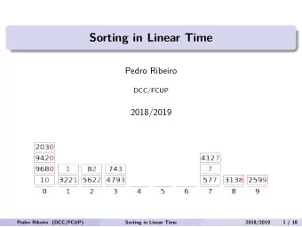
Radix Sort ➢ Sort on digits of the numbers, least significant digits first , with a stable sort algorithm, i.e., counting sort. ➢ Radix-sort(A,d): // d digits for i:=1 to d do sort_stable A on digit i ➢ If we sort n d -digits numbers with each digit taking k values (i.e. base k ), the running time is Θ (d(n+k)). ➢ Careful of the constants for comparison + it is not an in-place sorting algorithm. 5

Bucket Sort ➢ Assumes the input is uniformly distributed. ➢ Assumes the input in [0,1) ➢ bucket-sort(A): n:=length(A) for i:=1 to n do insert A[i] into list B[nA[i]] for i:=0 to n-1 do insertion_sort list B[i] concatenate lists B[0], B[1], ...,B[n-1] n − 1 T  n = n  ∑ i = 0 ➢ Running time: O  n i 2  ➢ Expected running time: Θ (n). 6