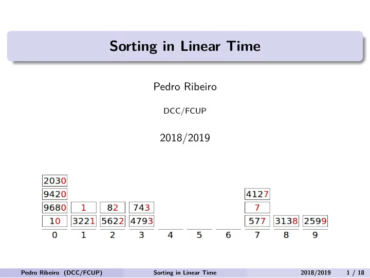
Sorting in Linear Time Pedro Ribeiro DCC/FCUP 2018/2019 Pedro - PowerPoint PPT Presentation

Sorting in Linear Time Pedro Ribeiro DCC/FCUP 2018/2019 Pedro Ribeiro (DCC/FCUP) Sorting in Linear Time 2018/2019 1 / 18

Sorting with and without comparisons We have already talked about several algorithms for sorting They were based on comparisons : questions of the form ” a < b ?” ◮ Quicksort ◮ Mergesort ◮ There are others such as Heapsort, ... We have shown that for these comparison-based algorithms we have a lower bound on the number of comparisons needed: Θ( n log n ) Today we are going to talk about algorithms not based on comparisons (and thus not restricted to the previous lower bound) Pedro Ribeiro (DCC/FCUP) Sorting in Linear Time 2018/2019 2 / 18

Counting Sort Assumption: integers to be sorted are in the range 0 to k Counting Sort - Sort elements in A , with sorted output in B CountingSort(A,B,k) : C[0..k] ← new array for i = 0 to k C[i] = 0 for i = 1 to A.length C[A[i]] = C[A[i]] + 1 // C [ i ] now contains the number of elements equal to i . for i = 1 to k C[i] = C[i] + C[i-1] // C [ i ] now contains the number of elements less than or equal to i . for i = A.length downto 1 B[C[A[i]]] = A[i] C[A[i]] = C[A[i]] -1 Pedro Ribeiro (DCC/FCUP) Sorting in Linear Time 2018/2019 3 / 18

Counting Sort (a) A and C after first counting loop (b) C after third loop (c) , (d) and (e) first iterations of last loop (f) final state of array B (figure from CLRS) Pedro Ribeiro (DCC/FCUP) Sorting in Linear Time 2018/2019 4 / 18

Counting Sort What is the time complexity ? Let n = A . length First loop: Θ( k ) Second loop: Θ( n ) Third loop: Θ( k ) Fourth loop: Θ( n ) Total: Θ( n + k ) If k is O ( n ) then this sort runs in linear time ! Θ( n ) Pedro Ribeiro (DCC/FCUP) Sorting in Linear Time 2018/2019 5 / 18

Stable sorting Stable sorting A sorting algorithm is said to be stable if in case of a tie it keeps the order of the original array This property may be important, for instance, when ”satellite” data is carried around the elements being sorted ◮ Ex: sorting persons - tuples (name, age) - only by age Counting Sort is stable! (because of the order of the last loop) ◮ This is why it may be used as a subroutine in Radix Sort, as we’ll see Pedro Ribeiro (DCC/FCUP) Sorting in Linear Time 2018/2019 6 / 18

Radix Sort Imagine you are sorting ”by columns” , i.e., by considering at a time each possible digit position Intuitively, you would probably imagine starting with the most significant digit . RadixSort solves the sorting problem somehow ”counter-intuitively”, by starting with the least significant digit . Pedro Ribeiro (DCC/FCUP) Sorting in Linear Time 2018/2019 7 / 18

Radix Sort Assumption: each element in the array A has d digits, where 1 is the lowest order digit, and d the highest-order digit Radix Sort RadixSort(A,d) : for i = 1 to d Use a stable sort to sort array A on digit i (figure from CLRS) Pedro Ribeiro (DCC/FCUP) Sorting in Linear Time 2018/2019 8 / 18

Radix Sort Radix Sort is akin to sorting by different fields ◮ Ex: sort dates by year, then by month, then by day We could do a comparison-based sort: compare year, if tie, compare month, if tie compare day or do 3 consecutive stable sorts: first by day, then by month, and finally by year Complexity of Radix Sort depends on the used sorting algorithm An usual choice is... Counting Sort! In this case we have Θ( d ( k + n )) ◮ We can sort n b -bit numbers in Θ(( b / r )( n + 2 r )) with counting sort ⋆ Each key has ⌈ b / r ⌉ digits of r bits each (our d ) ⋆ Each digit is an integer in the range 0 to 2 r − 1 (our k ) Pedro Ribeiro (DCC/FCUP) Sorting in Linear Time 2018/2019 9 / 18

Sorting Keys that are not numerical Counting and Radix sort do not depend on having numerical keys They depend on having the possibility to ”break” the key into ”digits” (parts) and to map each part into a numerical value For instance, if we have strings , we can break by chars, and map each char into a number ( a = 0 , b = 1 , . . . , z = 25) EAR SEA EAR BOX COW DOG SEA COW DOG BIG DIG DIG NOW -> EAR -> DOG -> DOG SEA COW COW EAR BOX NOW NOW FOX BIG BOX BOX NOW FOX FOX FOX SEA Pedro Ribeiro (DCC/FCUP) Sorting in Linear Time 2018/2019 10 / 18

Bucket Sort Assumption: keys follow an uniform distribution over a certain range Idea: make n equal sized ”buckets” , distribute input over buckets, sort each bucket and then concatenate results Rationale: If the input is uniformly distributed, than there will not be many numbers in each bucket ! Pedro Ribeiro (DCC/FCUP) Sorting in Linear Time 2018/2019 11 / 18

Bucket Sort Without loss of generality, let’s assume for now that the range is 0 .. 1 Bucket Sort - each bucket is a list BucketSort(A) : n = A.length B[0..n.1] ← new array of lists for i = 0 to n-1 B[i] = empty list for i = 1 to n insert A[i] into B[ ⌊ nA [ i ] ⌋ ] for i = 0 to n-1 sort list B[i] concatenate lists B[0], B[1], ..., B[n-1] together, in order Pedro Ribeiro (DCC/FCUP) Sorting in Linear Time 2018/2019 12 / 18

Bucket Sort An example (figure from CLRS) Pedro Ribeiro (DCC/FCUP) Sorting in Linear Time 2018/2019 13 / 18

Bucket Sort What is the execution time ? Everything except the cycle with sorts takes Θ ( n ) We need to analyse the time taken by the sorts Let’s assume we use Insertion Sort (good for lists) - each is O ( n 2 ) Execution Time of Bucket Sort (with Insertion Sort) n i : random variable denoting the number of elements in bucket i n − 1 O ( n 2 T ( n ) = Θ( n ) + � i ) i =0 Pedro Ribeiro (DCC/FCUP) Sorting in Linear Time 2018/2019 14 / 18

Bucket Sort We want to analyse the average-case running time of bucket sort: calculate the expected value of running time. n − 1 O ( n 2 E [ T ( n )] = E [Θ( n ) + � i )] i =0 n − 1 E [ O ( n 2 = Θ( n ) + � i )] (by linearity of expectation) i =0 n − 1 O ( E [ n 2 = Θ( n ) + � i ]) i =0 What is the value of E [ n 2 i ]? (expected size of each bucket i ) Pedro Ribeiro (DCC/FCUP) Sorting in Linear Time 2018/2019 15 / 18

Bucket Sort Claim: E [ n 2 i ] = 2 − 1 / n Let’s define an indicator random variable X ij with values: 1 if A [ j ] falls on bucket i , 0 otherwise n With this, n i = � X ij j =1 n E [ n 2 X ij ) 2 ] i ] = E [( � j =1 n n = E [ � � X ij X ik ] j =1 k =1 n X 2 = E [ � ij + � � X ij X ik ] j =1 1 ≤ j ≤ n 1 ≤ k ≤ n , k � = j n E [ X 2 = ij ] + E [ X ij X ik ] � � � j =1 1 ≤ j ≤ n 1 ≤ k ≤ n , k � = j Pedro Ribeiro (DCC/FCUP) Sorting in Linear Time 2018/2019 16 / 18

Bucket Sort Let’s first solve E [ X 2 ij ]. The probability of j being in bucket i is 1 / n , since the keys are uniformly distributed. ij ] = 1 2 × 1 n + 0 2 × (1 − 1 E [ X 2 n ) = 1 n Now, when k � = j , variables X ij and X ik are independent: E [ X ij X ik ] = E [ X ij ] E [ X ik ] = 1 n × 1 n = 1 n 2 Finally: n 1 1 E [ n 2 i ] = n + � � � n 2 j =1 1 ≤ j ≤ n 1 ≤ k ≤ n , k � = j n × 1 n + n ( n − 1) × 1 = n 2 1 + n − 1 = n 2 − 1 = n Pedro Ribeiro (DCC/FCUP) Sorting in Linear Time 2018/2019 17 / 18

Bucket Sort We want to analyse the average-case running time of bucket sort: calculate the expected value of running time. n − 1 O ( E [ n 2 E [ T ( n )] = Θ( n ) + i ]) � i =0 = Θ( n ) + n × O (2 − 1 / n ) = Θ( n ) Hence, Bucket Sort will have linear complexity on the average-case! Even if the input does not follow a uniform distribution, bucket sort may still run in linear time, as long as the sum of the squares of the bucket sizes is linear in the total number of elements. Pedro Ribeiro (DCC/FCUP) Sorting in Linear Time 2018/2019 18 / 18