Statistical Analysis of Corpus Data with R You shall know a word by - PowerPoint PPT Presentation

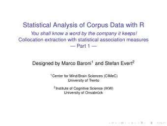
Statistical Analysis of Corpus Data with R You shall know a word by the company it keeps! Collocation extraction with statistical association measures — Part 2 — Designed by Marco Baroni 1 and Stefan Evert 2 1 Center for Mind/Brain Sciences (CIMeC) University of Trento 2 Institute of Cognitive Science (IKW) University of Onsabrück

Outline Scaling up: working with large data sets Statistical association measures Sorting and ranking data frames The evaluation of association measures Precision/recall tables and graphs MWE evaluation in R

Scaling up ◮ We know how to compute association scores ( X 2 , Fisher, and log θ ) for individual contingency tables now . . .

Scaling up ◮ We know how to compute association scores ( X 2 , Fisher, and log θ ) for individual contingency tables now . . . . . . but we want to do it automatically for 24,000 bigrams in the Brown data set, or an even larger number word pairs

Scaling up ◮ We know how to compute association scores ( X 2 , Fisher, and log θ ) for individual contingency tables now . . . . . . but we want to do it automatically for 24,000 bigrams in the Brown data set, or an even larger number word pairs ◮ Of course, you can write a loop (if you know C/Java): > attach(Brown) > result <- numeric(nrow(Brown)) > for (i in 1:nrow(Brown)) { if ((i %% 100) == 0) cat(i, " bigrams done\n") A <- rbind(c(O11[i],O12[i]), c(O21[i],O22[i])) result[i] <- chisq.test(A)$statistic } ☞ fisher.test() is even slower . . .

Vectorising algorithms ◮ Standard iterative algorithms (loops, function calls) are excruciatingly slow in R ◮ R is an interpreted language designed for interactive work and small scripts, not for implementing complex algorithms ◮ Large amounts of data can be processed efficiently with vector and matrix operations ➪ vectorisation ◮ even computations involving millions of numbers are carried out instantaneously ◮ How do you store a vector of contingency tables?

Vectorising algorithms ◮ Standard iterative algorithms (loops, function calls) are excruciatingly slow in R ◮ R is an interpreted language designed for interactive work and small scripts, not for implementing complex algorithms ◮ Large amounts of data can be processed efficiently with vector and matrix operations ➪ vectorisation ◮ even computations involving millions of numbers are carried out instantaneously ◮ How do you store a vector of contingency tables? ☞ as vectors O 11 , O 12 , O 21 , O 22 in a data frame

Vectorising algorithms ◮ High-level functions like chisq.test() and fisher.test() cannot be applied to vectors ◮ only accept a single contingency table ◮ or vectors of cross-classifying factors from which a contingency table is built automatically

Vectorising algorithms ◮ High-level functions like chisq.test() and fisher.test() cannot be applied to vectors ◮ only accept a single contingency table ◮ or vectors of cross-classifying factors from which a contingency table is built automatically ◮ Need to implement association measures ourselves ◮ i.e. calculate a test statistic or effect-size estimate to be used as an association score ➪ have to take a closer look at the statistical theory

Outline Scaling up: working with large data sets Statistical association measures Sorting and ranking data frames The evaluation of association measures Precision/recall tables and graphs MWE evaluation in R

Observed and expected frequencies w 2 ¬ w 2 w 2 ¬ w 2 E 11 � R 1 C 1 E 12 � R 1 C 2 w 1 O 11 O 12 � R 1 w 1 N N E 21 � R 2 C 1 E 22 � R 2 C 2 ¬ w 1 O 21 O 22 � R 2 ¬ w 1 N N � C 1 � C 2 � N ◮ R 1 , R 2 are the row sums ( R 1 = marginal frequency f 1 ) ◮ C 1 , C 2 are the column sums ( C 1 = marginal frequency f 2 ) ◮ N is the sample size ◮ E ij are the expected frequencies under independence H 0

Adding marginals and expected frequencies in R # first, keep R from performing integer arithmetic > Brown <- transform(Brown, O11=as.numeric(O11), O12=as.numeric(O12), O21=as.numeric(O21), O22=as.numeric(O22)) > Brown <- transform(Brown, R1=O11+O12, R2=O21+O22, C1=O11+O21, C2=O12+O22, N=O11+O12+O21+O22) # we could also have calculated them laboriously one by one: Brown$R1 <- Brown$O11 + Brown$O12 # etc.

Adding marginals and expected frequencies in R # first, keep R from performing integer arithmetic > Brown <- transform(Brown, O11=as.numeric(O11), O12=as.numeric(O12), O21=as.numeric(O21), O22=as.numeric(O22)) > Brown <- transform(Brown, R1=O11+O12, R2=O21+O22, C1=O11+O21, C2=O12+O22, N=O11+O12+O21+O22) # we could also have calculated them laboriously one by one: Brown$R1 <- Brown$O11 + Brown$O12 # etc. > Brown <- transform(Brown, E11=(R1*C1)/N, E12=(R1*C2)/N, E21=(R2*C1)/N, E22=(R2*C2)/N) # now check that E11, . . . , E22 always add up to N!

Statistical association measures Measures of significance ◮ Statistical association measures can be calculated from the observed, expected and marginal frequencies

Statistical association measures Measures of significance ◮ Statistical association measures can be calculated from the observed, expected and marginal frequencies ◮ E.g. the chi-squared statistic X 2 is given by ( O ij − E ij ) 2 � chi-squared = E ij ij (you can check this in any statistics textbook)

Statistical association measures Measures of significance ◮ Statistical association measures can be calculated from the observed, expected and marginal frequencies ◮ E.g. the chi-squared statistic X 2 is given by ( O ij − E ij ) 2 � chi-squared = E ij ij (you can check this in any statistics textbook) ◮ The chisq.test() function uses a different version with Yates’ continuity correction applied: � 2 � chi-squared corr = N | O 11 O 22 − O 12 O 21 | − N / 2 R 1 R 2 C 1 C 2

Statistical association measures Measures of significance ◮ P-values for Fisher’s exact test are rather tricky (and computationally expensive) ◮ Can use likelihood ratio test statistic G 2 , which is less sensitive to small and skewed samples than X 2 (Dunning 1993, 1998; Evert 2004) ◮ G 2 uses same scale (asymptotic χ 2 1 distribution) as X 2 , but you will notice that scores are entirely different O ij log O ij � log-likelihood = 2 E ij ij

Significance measures in R # chi-squared statistic with Yates’ correction > Brown <- transform(Brown, chisq = N * (abs(O11*O22 - O12*O21) - N/2)^2 / (R1 * R2 * C1 * C2) ) # Compare this to the output of chisq.test() for some bigrams. # What happens if you do not apply Yates’ correction?

Significance measures in R # chi-squared statistic with Yates’ correction > Brown <- transform(Brown, chisq = N * (abs(O11*O22 - O12*O21) - N/2)^2 / (R1 * R2 * C1 * C2) ) # Compare this to the output of chisq.test() for some bigrams. # What happens if you do not apply Yates’ correction? > Brown <- transform(Brown, logl = 2 * ( O11*log(O11/E11) + O12*log(O12/E12) + O21*log(O21/E21) + O22*log(O22/E22) )) > summary(Brown$logl) # do you notice anything strange?

Significance measures in R Watch your numbers! ◮ log 0 is undefined, so G 2 cannot be calculated if any of the observed frequencies O ij are zero ◮ Why are the expected frequencies E ij unproblematic?

Significance measures in R Watch your numbers! ◮ log 0 is undefined, so G 2 cannot be calculated if any of the observed frequencies O ij are zero ◮ Why are the expected frequencies E ij unproblematic? ◮ For these terms, we can substitute 0 = 0 · log 0 > Brown <- transform(Brown, logl = 2 * ( ifelse(O11>0, O11*log(O11/E11), 0) + ifelse(O12>0, O12*log(O12/E12), 0) + ifelse(O21>0, O21*log(O21/E21), 0) + ifelse(O22>0, O22*log(O22/E22), 0) )) # ifelse() is a vectorised if -conditional

Effect-size measures ◮ Direct implementation allows a wide variety of effect size measures to be calculated ◮ but only direct maximum-likelihood estimates, confidence intervals are too complex (and expensive) ◮ Mutual information and Dice coefficient give two different perspectives on collocativity: O 11 2 O 11 MI = log 2 Dice = E 11 R 1 + C 1 ◮ Modified log odds ratio is a reasonably good estimator: odds-ratio = log ( O 11 + 1 2 )( O 22 + 1 2 ) ( O 12 + 1 2 )( O 21 + 1 2 )

Further reading ◮ There are many other association measures ◮ Pecina (2005) lists 57 different measures ◮ Evert, S. (to appear). Corpora and collocations. In A. Lüdeling and M. Kytö (eds.), Corpus Linguistics. An International Handbook , article 57. Mouton de Gruyter, Berlin. ◮ explains characteristic properties of the measures ◮ contingency tables for textual and surface cooccurrences ◮ Evert, Stefan (2004). The Statistics of Word Cooccurrences: Word Pairs and Collocations . Dissertation, Institut für maschinelle Sprachverarbeitung, University of Stuttgart. Published in 2005, URN urn:nbn:de:bsz:93-opus-23714. ◮ full sampling models and detailed mathematical analysis ◮ Online repository: www.collocations.de/AM ◮ with reference implementations in the UCS toolkit software ☞ all these sources use the notation introduced here

Implementiation of the effect-size measures # Can you compute the association scores without peeking ahead?