Spectral analysis of ZUC-256 The algorithm of ZUC-256 Attack - PowerPoint PPT Presentation
Spectral analysis of ZUC-256 The algorithm of ZUC-256 Attack approaches Spectral analysis tools 5G future is here! Alexander Maximov Ericsson Research, Lund, Sweden Jing Yang and Thomas Johansson Lund University, Lund, Sweden Fast
Spectral analysis of ZUC-256 • The algorithm of ZUC-256 • Attack approaches • Spectral analysis tools 5G future is here! Alexander Maximov Ericsson Research, Lund, Sweden Jing Yang and Thomas Johansson Lund University, Lund, Sweden Fast Software Encryption 2020, November 9-13
Introduction of ZUC-128/256 ●Domestic cipher used in China ●32-bit oriented stream cipher ●FSM over GF(2 32 ) ●LFSR over prime modulo p=2 31 -1 ●BR layer ●[2011] 3GPP standard UEA3/UIA3 with 128-bit key ●[2018] ZUC-256 was proposed as a 256-bit key version for 5G air encryption ● Eurocrypt 2018 Rump session ● ZUC-256 Workshop ●No attack faster than 2 256 found (until now) ●We propose an academic attack 2 20 faster than exhaustive key search
Linear approximation: Z p 2xGF(2 16 ) ●Start from the LFSR and BR layer ●Approximate as 2xGF(2 16 ) ●Example: for
Linear approximation: Deriving biased samples ●Two consecutive keystream words ● New idea: Include LFSR cancellation into the full noise expression, thus making the bias larger ●σ – swap of high and low 16 bits ● M – 32x32 Boolean matrix that the attacker can choose
Academic distinguishing attack: Results ● Sampling ● Problem 1: ●Computation of 32-bit ● Total noise expression (details on N1 and N2 will be given later) noise distributions (adapted “bit-slicing” technique) ● Problem 2: ● Found matrix M ●Searching for the 32x32 binary masking matrix M (spectral analysis) ● Bias of the total noise (Squared Euclidean Imbalance, SEI) ● Distinguishing attack complexity is O(1/ε) = O(2 236 ) the degree is ~2 167 ●in
Noise expressions and “Bit-slicing” technique ●Problem: ●32-bit noise variables ●Just computing Dist(N1a) would require a loop of size 9 3 * 2 17*32 ! ●Solution: ●Compute with adapted “Bit-slicing” technique in time ~O(2 47 ).
Problem 2: Searching for the linear masking matrix M ●Recall the total noise expression: ●Assume we have computed the distributions of 32-bit noise variables N1 and N2. ● Problem: How to find a good 32x32 binary matrix M and to maximize the total bias? ● Solution: Spectral analysis techniques (next slides)
Spectral tools: Introduction ●n-bit variables, size of the alphabet ●t- random variables (noise variables) ●For a random variable X, individual values are ●WHT and DFT ●What can we do in frequency domain for cryptanalysis? ●Bias computation and precision problem ●Convolutions of noise distributions ●Search for a linear masking (e.g. nxn binary matrix M) ●Approximation of S-Boxes ●…etc
Spectral tools: Bias computation and precision problem ● Problem: if expected bias is ~2 -p then in ●Bias = Squared Euclidean Imbalance ( f = normalization factor) time domain the values must have precision at least O(|p/2|) bits! ●Example: for an expected bias 2 -512 we must ●A distinguisher needs samples handle large number arithmetic and have precision >256 bits. ● Theorem 1: bias computation in the frequency domain Consequences ●In the frequency domain only low precision is needed, but with the exponent field ●Data type double in standard C is good enough (exponent value up to 2 -1023 ) ●Works even if the initial distribution of X is not normalized (then f is used)
Spectral tools: Convolutions ●From e.g. [MJ05] ●Consequence: the bias of a convolution Observation & Motivation ●Peak spectrum values contribute the most to the total bias ●Motivates to learn how to “shuffle” spectrums by some manipulations in the time domain.
Spectral tools: Linear masking (WHT case) ● ● Theorem 2: ● Algorithm 1: (solution to find M-matrices above) ●Place wanted n indexes as rows of the matrix (must be full rank) ●For each find n spectral indexes with peak spectral values (sorted descending order). Place those indexes as rows of (must be full rank) ●Derive
Spectral tools: Linear masking (DFT case) ● ● Theorem 6: ● Cor. 2&3: ● Algorithm 3: (solution to find c-constants above) ●Locate the “group” m where the maximum peak value is happening over the product of group-max values for all Xs ●Set such that it “rotates” the corresponding spectrum within the group m ●Best alignment happens at the point 2 m
Spectral tools: Approximation of S-Boxes (Intro) ●Examples for composite S-Box constructions: ●Example of an approximation: ● Questions: ●How to find M such that the bias of X is large? ●How to derive the spectrum value of X at index k?
Spectral tools: Usual S-Boxes ● ● Theorem 3: ● Algorithm 2: (Find a good masking matrix M) ●for each k>0 compute WHT: ●loop for λ-index over the k-th spectrum above ●collect many enough triples ●from the triples construct full-rank matrices with greedy approach ●derive
Spectral tools: Composite S-Boxes ● Theorem 5: ● Usage example: ●for all basic S-Boxes (8-bit S0/S1 in ZUC) precompute tables like ●then any spectrum values of a large composite S-Box can be derived through these tables:
Spectral analysis of ZUC –the final step! ●Recall the total noise expression: ●For any point k, the spectral expression for the total noise: ● Spectral analysis of ZUC: our strategy for the final step to find M ●we selected ~2 24.78 “promising” λ-points where ●we selected ~2 18 “promising” k-points where ●for each pair (k, λ) we compute the spectrum value, then collect best pairs (k, λ) ●construct matrices and derive
Bit-slicing technique: Basics ● N1a, N1b, N2 are 32-bit noise variables: ●have 32-bit operators ●2x16-bit operators ●the carry random variables C = {0, -1, +1}. ●Consider a 32-bit “toy” noise expression N (we use the same techniques to compute N1a, N1b, N2). ● Table k (c1, c2…) = number of combinations of k-bit truncated input variables (X1, X2…) such that the result is a wanted k-bit truncated result R and the output sub-carries are c1 and c2 . ●Given Table k (c1, c2…) and r k it is easy to compute Table k+1 (c1, c2…) ●Transition from k’th table to (k+1)’th is a linear operation => transition matrices M x , where x=r k . ● Table k (c1, c2…) vector V k of length t .
Bit-slicing technique: Basics ●Two transition matrices can be precomputed: ●General formulae: ●Precomputation of high and low parts.
Bit-slicing technique: Adaptation ●C 0 and C 16 are independent variables in range {0, -1, +1} with certain probabilities. ●Table’s entries are #of combinations * Pr{C 0 , C 16 } ●Special transition matrices for bits 0, 15, 16 ●Transition matrices are of size 2 12.8 x2 12.8 (365Mb of RAM each) ●L/H vectors: ●truncated lengths t=2 8 . ●precomputation time O(2 46.6 )
Recommend
More recommend
Explore More Topics
Stay informed with curated content and fresh updates.
