Sparse plus low-rank graphical models of time series Presented by - PowerPoint PPT Presentation
Sparse plus low-rank graphical models of time series Presented by Rahul Nadkarni Joint work with Nicholas J. Foti, Adrian KC Lee, and Emily B. Fox University of Washington August 14 th , 2016 1 Brain Interactions from MEG
Sparse plus low-rank graphical models of time series Presented by Rahul Nadkarni Joint work with Nicholas J. Foti, Adrian KC Lee, and Emily B. Fox University of Washington August 14 th , 2016 1
Brain Interactions from MEG Magnetoencephalography (MEG) captures weak magnetic field. Goal: Infer functional connectivity 2
Graphical Models • Graph G= ( V, E ) encodes conditional independence statements. nodes edges No edge ( i, j ) X i , X j conditionallyindependent ↔ given rest of variables. ⊥ X 2 | X 3 , X 4 , X 5 X 1 ⊥ 3
Graphical Models of Time Series No edge ( i,j ) time series X i , X j conditionallyindependent ⇒ given entire trajectories of other series. Accounts for interactions at all lags . • Removes linear effects of other series. • Natural property for functional connectivity Examples of existing work: Bach et al. 2004, Songsiri & Vandenberghe 2010, Jung et al. 2015, Tank et al. 2015 4
Latent structure latent variables marginalized over latent variables latent component observed component + observed variables Examples of existing work: Chandrasekaran et al. 2012, Jalali & Sanghavi 2012, Liégois et al. 2015 5
Encoding graph structure 6
Gaussian random vectors X ∼ N (0 , Σ ) • For Gaussian random vector Conditional independenceencoded in the precision matrix. Σ − 1 = ⇐⇒ X i , X j conditionallyindependentgiven rest of variables. 7
Gaussian stationary processes lagged covariance: X 1 ( t ) Γ ( h ) = Cov( X ( t ) , X ( t + h )) X 2 ( t ) . . . . ? . . Γ ( h ) X p ( t ) How is conditional independence encoded? 8
Model in the Frequency Domain d k X ( t ) FFT Spectral density matrix Lagged covariance matrix as the Fourier transform of the ∞ X Γ ( h ) e − i λ h S ( λ ) = matrices, Γ ( h ) = Cov ( X ( t ) , X ( t + h )) : h = −∞ 9
Encoding structure in frequency domain For Gaussian i.i.d. random variables, �� �� �� �� �� Σ − 1 = �� �� �� �� �� �� �� �� �� �� �� ( Dahlhaus, 2000 ) For Gaussian stationary time series, S ( λ ) − 1 : �� �� �� �� �� �� �� �� �� �� �� �� �� �� �� �� �� �� �� �� �� �� �� �� �� �� �� �� �� �� �� �� �� �� �� �� �� �� �� �� �� �� �� �� �� �� �� �� �� �� �� �� �� �� �� �� �� �� �� �� �� �� �� �� �� �� �� �� �� �� �� �� �� �� �� �� �� �� �� �� �� �� �� �� �� �� �� �� �� �� �� �� �� �� �� �� �� �� �� �� �� �� �� �� �� �� �� �� �� �� �� �� �� �� �� �� �� �� �� �� �� �� �� �� �� �� �� �� �� �� �� �� �� �� �� �� �� �� �� �� �� �� �� �� �� �� �� �� �� �� �� �� �� �� �� �� �� �� �� �� λ 1 λ 2 λ k λ T . . . . . . complex inverse sp spectral densi sity matrices 10
Learning structure from data 11
Penalized likelihood expression inverse covariance matrix + − log (Likelihood( Ψ )) λ · Penalty( Ψ ) sample covariance matrix n o X | Ψ ij | ˆ − log det Ψ + tr S Ψ i<j negative log-likelihood of Gaussian sparsity-inducing penalty Graphical LASSO (Friedman et al. 2007) solved with: many existing algorithms What’s our likelihood in the frequency-domain case? 12
Likelihood in the Frequency Domain Time Domain Likelihood Frequency Domain Likelihood p ( d 0 , . . . , d T − 1 |{ S ( λ k ) } T − 1 p ( X (1) , . . . , X ( T ) | [ Γ ( h )] T − 1 k =0 ) h =0 ) Fourier coefficients Fourier coefficients are asymptotically independent, complex Normal random vectors (Brillinger, 1981) Whittle Approximation S k ≡ S ( λ k ) T − 1 1 k S − 1 Y π p | S k | e − d ∗ p ( d 1 , . . . , d T |{ S ( λ k ) } T − 1 d k k =0 ) ≈ k k =0 13
Penalized likelihood expression in frequency domain inverse spectral density matrix T − 1 ! 1 k S − 1 Y π p | S k | e − d ∗ d k + − log λ · Penalty( Ψ ) k k =0 sample spectral density matrix v T − 1 T − 1 u ⇣ n o ⌘ ˆ X X u X − log det Ψ [ k ] + tr S [ k ] Ψ [ k ] | Ψ [ k ] ij | 2 t i<j k =0 k =0 Group LASSO penalty Spectral graphical LASSO (Jung et al. 2015) solved with: ADMM (Jung et al. 2015) 14
Incorporating latent processes 15
Latent structure in MEG latent variables • MEG recordings affected by neural activity unrelated to task • Mapping from recordings to brain activity introduces “point spread” These issues can be addressed by adding a latent component to the model observed variables 16
Sparse plus low-rank decomposition observed-hidden p r observed-observed � K OO K OH S − 1 = K = = K HO K HH hidden-observed hidden-hidden -1 – ⨉ ⨉ K O = sparse low-rank (rank r << p) 17
Sparse plus low-rank penalized likelihood -1 – ⨉ ⨉ Ψ L negative log-likelihood: n o ˆ − log det( Ψ − L ) + tr S ( Ψ − L ) sparse penalty: low-rank penalty: X tr { } | | ij -1 ⨉ ⨉ i<j Latent variable GLASSO (Chandrasekaran et al. 2012) solved with ADMM (Ma et al. 2013) 18
Latent variable spectral GLASSO negative log-likelihood: T − 1 ⇣ n o ⌘ X ˆ − log det( Ψ [ k ] − L [ k ]) + tr S [ k ]( Ψ [ k ] − L [ k ]) k =0 Whittle approximation low-rank penalty: sparse penalty: v T − 1 T − 1 u X tr { L [ k ] } X u X | Ψ [ k ] ij | 2 t k =0 i<j k =0 Group LASSO penalty Used ADMM to solve this convex formulation 19
Analysis pipeline graph Multivariate time series data Estimated spectral density ADMM sparse component: low-rank component: time domain frequency domain 20
Synthetic data results 21
MEG Auditory Attention Analysis Maintain or Switch attention (Left/Right, High/Low pitch) 16 subjects, 10-50 trials each. • Each trial results in a 149-dimensional time series. • 22
Summary graph sparse component: low-rank component: • Frequency domain for conditional independence structure and likelihood • Modeling latent component gives sparser, more interpretable graphs • Latent variable, spectral models are important in neuroscience 23
Recommend
More recommend
Explore More Topics
Stay informed with curated content and fresh updates.
