Frequency Synthesizers for RF Transceivers Modelling of PLL in the - PowerPoint PPT Presentation

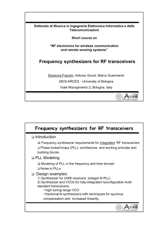
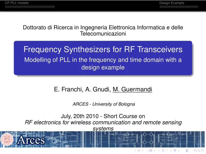
CP-PLL models Design Example Dottorato di Ricerca in Ingegneria Elettronica Informatica e delle Telecomunicazioni Frequency Synthesizers for RF Transceivers Modelling of PLL in the frequency and time domain with a design example E. Franchi, A. Gnudi, M. Guermandi ARCES - University of Bologna July, 20th 2010 - Short Course on RF electronics for wireless communication and remote sensing systems

CP-PLL models Design Example Outline 1 CP-PLL models The need for accurate PLL models s-domain model z-domain model Time-domain model Comparison between models Phase Noise Models 2 Design Example: Frequency Synthesizer for UWB MB-OFDM UWB communications Synthesizer Architecture PLLs Tuning Range Extension Measured results

CP-PLL models Design Example Outline 1 CP-PLL models The need for accurate PLL models s-domain model z-domain model Time-domain model Comparison between models Phase Noise Models 2 Design Example: Frequency Synthesizer for UWB MB-OFDM UWB communications Synthesizer Architecture PLLs Tuning Range Extension Measured results

CP-PLL models Design Example Charge Pump Phase Locked Loops (CP-PLLs) F REF PHASE UP F REF CHARGE LOOP OUT FREQ VCO DN PUMP FILTER DETECTOR F FREQ DIV DIVIDER Charge Pump Phase Locked Loop PFD-CP compares phase misalignment between feedback and reference signal. Loop Filter integrates error signal and controls VCO output frequency. When in-lock F OUT = N · F REF . Loop tracks phase and frequency misalignments with zero errors.

CP-PLL models Design Example Charge Pump Phase Locked Loops (CP-PLLs) F REF PHASE UP F REF CHARGE LOOP OUT FREQ VCO DN PUMP FILTER DETECTOR F FREQ DIV DIVIDER Charge Pump Phase Locked Loop CP , LF and VCO are continuous-time systems. PFD and FD are edge-driven systems. Phase comparison is performed once per reference period, not continuously.

CP-PLL models Design Example The need for accurate PLL models PLL models Simulations need to be performed hierarchically. Circuit level time-domain simulation is not feasible.

CP-PLL models Design Example The need for accurate PLL models PLL models Simulations need to be performed hierarchically. Circuit level time-domain simulation is not feasible. Traditional models ( s-domain and z-domain ) rely on linearizations and approximations to simplify loop analysis.

CP-PLL models Design Example The need for accurate PLL models PLL models Simulations need to be performed hierarchically. Circuit level time-domain simulation is not feasible. Traditional models ( s-domain and z-domain ) rely on linearizations and approximations to simplify loop analysis. Efficient semi-analytical time-domain models can avoid these approximations, with reduced computation time.

CP-PLL models Design Example The need for accurate PLL models PLL models Simulations need to be performed hierarchically. Circuit level time-domain simulation is not feasible. Traditional models ( s-domain and z-domain ) rely on linearizations and approximations to simplify loop analysis. Efficient semi-analytical time-domain models can avoid these approximations, with reduced computation time. Derivation and comparison between these models is performed.

CP-PLL models Design Example Outline 1 CP-PLL models The need for accurate PLL models s-domain model z-domain model Time-domain model Comparison between models Phase Noise Models 2 Design Example: Frequency Synthesizer for UWB MB-OFDM UWB communications Synthesizer Architecture PLLs Tuning Range Extension Measured results

CP-PLL models Design Example Fourth order PLL s-domain model Approximation PFD CP LPF VCO θ r θ 2 π 1 K o Charge injected by charge G G (s) VCO s 2 π LF pump over one period: V C Q = θ r − θ d 2 π GT θ 1 d N FD REF Q C t DIV −3 π −2 π π − π π π ∆θ t 2 3 Icp t

CP-PLL models Design Example Fourth order PLL s-domain model Approximation PFD CP LPF VCO θ r θ 2 π 1 K o Charge injected by charge G G (s) VCO s 2 π LF pump over one period: V C Q = θ r − θ d 2 π GT θ 1 d N If the loop dynamic is slow FD enough one can neglect the CP current actual REF shape Q C t DIV −3 π −2 π π − π π π ∆θ t 2 3 Icp t

CP-PLL models Design Example Fourth order PLL s-domain model Approximation PFD CP LPF VCO θ r θ 2 π 1 K o Charge injected by charge G G (s) VCO s 2 π LF pump over one period: V C Q = θ r − θ d 2 π GT θ 1 d N If the loop dynamic is slow FD enough one can neglect the CP current actual REF shape Q C t and substitute it with an DIV −3 π −2 π π − average current: π π π ∆θ t 2 3 Icp i CP = G θ r − θ d t 2 π

CP-PLL models Design Example Fourth order PLL s-domain model Approximation PFD CP LPF VCO θ r θ 2 π 1 K o Charge injected by charge G G (s) VCO s 2 π LF pump over one period: V C Q = θ r − θ d 2 π GT θ 1 d N If the loop dynamic is slow FD enough one can neglect the CP current actual REF shape Q C t and substitute it with an DIV −3 π −2 π π − average current: π π π ∆θ t 2 3 Icp i CP = G θ r − θ d t 2 π Averaged linear continuous time PLL model

CP-PLL models Design Example s-domain model transfer functions CP-PFD i CP = G θ r − θ d I CP ( s ) θ r ( s ) − θ d ( s ) = G PFD CP LPF VCO → θ r 2 π 2 π θ 2 π 1 K o G G (s) VCO s 2 π LF V C θ 1 d N FD REF Q C t DIV −3 π −2 π π − π π π ∆θ t 2 3 Icp t

CP-PLL models Design Example s-domain model transfer functions CP-PFD i CP = G θ r − θ d I CP ( s ) θ r ( s ) − θ d ( s ) = G PFD CP LPF VCO → θ r 2 π 2 π θ 2 π 1 K o G G (s) VCO s 2 π LF V C 3 rd order LF θ 1 d G LF ( s ) = V C ( s ) N I CP ( s ) = FD s + 1 /τ z K LF s · ( s + b /τ z ) · ( s + c /τ z )

CP-PLL models Design Example s-domain model transfer functions CP-PFD i CP = G θ r − θ d I CP ( s ) θ r ( s ) − θ d ( s ) = G PFD CP LPF VCO → θ r 2 π 2 π θ 2 π 1 K o G G (s) VCO s 2 π LF V C 3 rd order LF θ 1 d G LF ( s ) = V C ( s ) N I CP ( s ) = FD s + 1 /τ z K LF s · ( s + b /τ z ) · ( s + c /τ z ) QVCO f o = K VCO · V C , θ o = � 2 π f o ( t ) dt → θ o ( s ) V C ( s ) = 2 π · K VCO s

CP-PLL models Design Example s-domain model transfer functions CP-PFD i CP = G θ r − θ d I CP ( s ) θ r ( s ) − θ d ( s ) = G PFD CP LPF VCO → θ r 2 π 2 π θ 2 π 1 K o G G (s) VCO s 2 π LF V C 3 rd order LF θ 1 d G LF ( s ) = V C ( s ) N I CP ( s ) = FD s + 1 /τ z K LF s · ( s + b /τ z ) · ( s + c /τ z ) QVCO f o = K VCO · V C , θ o = � 2 π f o ( t ) dt → θ o ( s ) V C ( s ) = 2 π · K VCO s FD θ d ( s ) θ o ( s ) = 1 N

CP-PLL models Design Example Fourth order PLL s-domain model PFD CP LPF VCO θ r θ 2 π 1 K o G G (s) VCO s 2 π LF V C 1 θ d N FD Open loop transfer function... G c ( s ) = G · K VCO · G LF ( s ) s · N

CP-PLL models Design Example Fourth order PLL s-domain model PFD CP LPF VCO θ r θ 2 π 1 K o G G (s) VCO s 2 π LF V C 1 θ d N FD ... for third order LF ... Open loop transfer function... G c ( s ) = G · K VCO · G LF ( s ) s + 1 /τ z G c ( s ) = K C s · N s 2 · ( s + b /τ z ) · ( s + c /τ z )

CP-PLL models Design Example Fourth order PLL s-domain model PFD CP LPF VCO θ r θ 2 π 1 K o G G (s) VCO s 2 π LF V C 1 θ d N FD ... for third order LF ... Open loop transfer function... G c ( s ) = G · K VCO · G LF ( s ) s + 1 /τ z s · N G c ( s ) = K C s 2 · ( s + b /τ z ) · ( s + c /τ z ) ... with K C = GK VCO K LF . N

CP-PLL models Design Example Fourth order PLL s-domain model PFD CP LPF VCO θ r θ 2 π 1 K o G G (s) VCO s 2 π LF V C 1 θ d N FD ... for third order LF ... Open loop transfer function... G c ( s ) = G · K VCO · G LF ( s ) s + 1 /τ z s · N G c ( s ) = K C s 2 · ( s + b /τ z ) · ( s + c /τ z ) Closed loop transfer function ... with θ o G · K VCO N · G LF ( s ) = K C = GK VCO K LF θ r s · N + G · K VCO · G LF ( s ) . N

CP-PLL models Design Example Fourth order PLL s-domain model Gc PFD 20log(| |) CP LPF VCO 1+Gc θ r θ Gc 2 π 1 K o G G (s) VCO s 2 π LF N V C 1 θ d N bfz cfz fz fc log f FD ... for third order LF ... Open loop transfer function... arg( ) G c ( s ) = G · K VCO · G LF ( s ) s + 1 /τ z s · N G c ( s ) = K C s 2 · ( s + b /τ z ) · ( s + c /τ z ) Closed loop transfer function log f ... with φ m θ o G · K VCO N · G LF ( s ) π = K C = GK VCO K LF θ r s · N + G · K VCO · G LF ( s ) . N

CP-PLL models Design Example Fourth order PLL s-domain model PFD CP LPF VCO Gc 20log(| |) θ r 1+Gc θ 2 π 1 K o Gc G G (s) VCO s 2 π LF V N C 1 θ d N bfz cfz FD fz fc log f ... for third order LF ... Open loop transfer function... G c ( s ) = G · K VCO · G LF ( s ) arg( ) s + 1 /τ z G c ( s ) = K C s · N s 2 · ( s + b /τ z ) · ( s + c /τ z ) Closed loop transfer function log f Rule of thumb for design φ θ o G · K VCO N · G LF ( s ) m � f step π = 1 � θ r s · N + G · K VCO · G LF ( s ) f c = t lock ζ e ( φ m ) ln f error