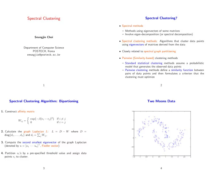
Spectral Clustering Spectral Clustering? Spectral methods Methods - PowerPoint PPT Presentation

Spectral Clustering Spectral Clustering? • Spectral methods – Methods using eigenvectors of some matrices – Involve eigen-decomposition (or spectral decomposition) Seungjin Choi • Spectral clustering methods: Algorithms that cluster data points using eigenvectors of matrices derived from the data Department of Computer Science POSTECH, Korea • Closely related to spectral graph partitioning seungjin@postech.ac.kr • Pairwise (Similarity-based) clustering methods – Standard statistical clustering methods assume a probabilistic model that generates the observed data points – Pairwise clustering methods define a similarity function between pairs of data points and then formulates a criterion that the clustering must optimize 1 2 Spectral Clustering Algorithm: Bipartioning Two Moons Data 1. Construct affinity matrix 1.5 � exp {− β � v i − v j � 2 } if i � = j W ij = 1 0 if i = j 0.5 2. Calculate the graph Laplacian L : L = D − W where D = diag { d 1 , . . . , d n } and d i = � j W ij . 0 3. Compute the second smallest eigenvector of the graph Laplacian (denoted by u = [ u 1 · · · u n ] ⊤ , Fiedler vector) −0.5 4. Partition u i ’s by a pre-specified threshold value and assign data points v i to cluster. −1 −1.5 −1 −0.5 0 0.5 1 1.5 2 2.5 3 3 4

Two Moons Data: k -Means Two Moons Data: Fiedler Vector 1.2 0.06 1 0.04 0.8 0.02 0.6 0 0.4 −0.02 0.2 0 −0.04 −0.2 −0.06 −0.4 −0.08 −0.6 −0.1 −0.8 0 20 40 60 80 100 120 140 160 180 200 −1.5 −1 −0.5 0 0.5 1 1.5 2 2.5 3 5 6 Two Moons Data: Spectral Clustering Graphs • Consider a connected graph G ( V , E ) where V = { v 1 , . . . , v n } and E 1.2 denote a set of vertices and a set of edges, respectively, with pairwise 1 similarity values being assigned as edge weights. 0.8 0.6 • Adjacency matrix (similarity, proximity, affinity matrix): W = [ W ij ] ∈ R n × n . 0.4 0.2 • Degree of nodes: d i = � j W ij . 0 • Volume: vol ( S 1 ) = d S 1 = � −0.2 i ∈S 1 d i . −0.4 −0.6 −0.8 −1.5 −1 −0.5 0 0.5 1 1.5 2 2.5 3 7 8

Neighborhood Graphs Graph Laplacian (Unnormalized) graph Laplacian is defined as L = D − W . Gaussian similarity function is given by 1. For every vector x ∈ R n , we have � � −� v i − v j � 2 w ( v i , v j ) = W ij = exp . n n � � x ⊤ Lx = 1 2 σ 2 W ij ( x i − x j ) 2 ≥ 0 . ( positive semidefinite ) 2 i =1 j =1 • ǫ -neighborhood graph 2. The smallest eigenvalue of L is 0 and the corresponding eigenvector • k -nearest neighbor graph is 1 = [1 · · · 1] ⊤ , since D 1 = W 1 , i.e, L 1 = 0 . 3. L has n nonnegative eigenvalues, λ 1 ≥ λ 2 ≥ · · · ≥ λ n = 0 . 9 10 Normalized Graph Laplacian Two different normalization methods are popular, including: x ⊤ Lx x ⊤ Dx − x ⊤ Wx = • Symmetric normalization: n n n � � � d i x 2 i − = W ij x i x j L s = D − 1 2 LD − 1 2 = I − D − 1 2 WD − 1 2 . i =1 i =1 j =1   � � � � 1 d i x 2 d j x 2  = i − 2 W ij x i x j + • Normalization related to random walks: j 2 i i j j � � L rw = D − 1 L = I − D − 1 W. 1 W ij ( x i − x j ) 2 . = 2 i j 11 12

1. For every vector x ∈ R n , we have Unnormalized Spectral Clustering � � 2 n n � � x ⊤ L s x = 1 x i − x j W ij √ d i � . 1. Construct a neighborhood graph with corresponding adjacency 2 d j matrix W . i =1 j =1 2. Compute the unnormalized graph Laplacian L = D − W . 2. L sym and L rw are positive semidefinite and have n nonnegative real-valued eigenvalues, λ 1 ≥ · · · λ n = 0 . 3. Find the k smallest eigenvectors of L and form the matrix U = [ u 1 · · · u k ] ∈ R n × k . 3. λ is an eigenvalue of L rw with eigenvector u if and only if λ is an eigenvalue of L s with eigenvector D 1 / 2 u . 4. Treating each row of U as a point in R k , cluster them into k groups using k -means algorithm. 4. λ is an eigenvalue of L rw with eigenvector u if and only if λ and u solves the generalized eigenvalue problem Lu = λDu . 5. Assign v i to cluster j if and only if row i of U is assigned to cluster j . 5. 0 is an eigenvalue of L rw with the constant one vector 1 as eigenvector. 0 is an eigenvalue of L s with eigenvector D 1 / 2 1 . 13 14 Normalized Spectral Clustering: Shi-Malik Normalized Spectral Clustering: Ng-Jordan-Weiss 1. Construct a neighborhood graph with corresponding adjacency 1. Construct a neighborhood graph with corresponding adjacency matrix W . matrix W . 2. Compute the normalized graph Laplacian L s = D − 1 / 2 LD − 1 / 2 . 2. Compute the unnormalized graph Laplacian L = D − W . 3. Find the k smallest eigenvectors u 1 , . . . , u k of L s and form the matrix U = [ u 1 · · · u k ] ∈ R n × k . 3. Find the k smallest generalized eigenvectors u 1 , . . . , u k of the problem Lu = λDu and form the matrix U = [ u 1 · · · u k ] ∈ R n × k . 4. Form the matrix � U from U by re-normalizing each row of U to have U ij = U ij / ( � unit norm, i.e., � j U ij ) 1 / 2 . 4. Treating each row of U as a point in R k , cluster them into k groups using k -means algorithm. 5. Treating each row of � U as a point in R k , cluster them into k groups using k -means algorithm. 5. Assign v i to cluster j if and only if row i of U is assigned to cluster j . 6. Assign v i to cluster j if and only if row i of � U is assigned to cluster j . 15 16

Where does this spectral clustering algorithm come Pictorial Illustration of Graph Partitioning from? • Spectral graph partitioning • Properties of block (diagonal) matrix • Markov random walk 17 18 Graph Partitioning: Bipartitioning Pictorial Illustration: Cut and Volume • Consider a connected graph G ( V , E ) where V = { v 1 , . . . , v n } and E denote a set of vertices and a set of edges, respectively, with pairwise similarity values being assigned as edge weights. • Graph bipartitioning involves taking the set V apart into two coherent = � + � groups, S 1 and S 2 , satisfying V = S 1 ∪S 2 , ( |V| = n ), and S 1 ∩S 2 = ∅ , � �� � �� � �� � cut ( S 1 , S 2 ) by simply cutting edges connecting the two parts vol ( S 1 ) vol ( S 2 ) • Adjacency matrix (similarity, proximity, affinity matrix): W = [ W ij ] ∈ R n × n . • Degree of nodes: d i = � j W ij . − � − � �� � �� � S 1 only S 2 only • Volume: vol ( S 1 ) = d S 1 = � i ∈S 1 d i . 19 20

Graph Partitioning Cut: Bipartitioning The task is to find k disjoint sets, S 1 , . . . , S k , given G = ( V , E ) , where The degree of dissimilarity between S 1 and S 2 can be computed by the total weights of edges that have been removed. S 1 ∩· · ·∩S k = φ and S 1 ∪· · ·∪S k = V such that a certain cut criterion is minimized. X X Cut ( S 1 , S 2 ) = W ij i ∈S 1 j ∈S 2 1. Bipartitioning: cut ( S 1 , S 2 ) = � � j ∈S 2 W ij . 8 9 i ∈S 1 1 < = X X X X X X = d i + d j − W ij − W ij 2. Multiway partitioning: cut ( S 1 , . . . , S k ) = � k 2 : i ∈S 1 j ∈S 2 i ∈S 1 j ∈S 1 i ∈S 2 j ∈S 2 ; i =1 cut ( S i , S i ) . 1 n ( q 1 − q 2 ) ⊤ L ( q 1 − q 2 ) o = , 3. Ratio cut: Rcut ( S 1 , . . . , S k ) = � k i =1 cut ( S i , S i ) 4 . |S i | where q j = [ q 1 j · · · q nj ] ⊤ ∈ R n is the indicator vector which represents partitions, 4. Normalized cut: Ncut ( S 1 , . . . , S k ) = � k i =1 cut ( S i , S i )  1 , vol ( S i ) . if i ∈ S j q ij = , for i = 1 , . . . , n and j = 1 , 2 . 0 , if i / ∈ S j Note that q 1 and q 2 are orthogonal, i.e., q ⊤ 1 q 2 = 0 . 21 22 Rcut and Unnormalized Spectral Clustering: k = 2 Introducing bipolar indicator vector, x = q 1 − q 2 ∈ { +1 , − 1 } n , the cut criterion is simplified as Define the indicator vector x = [ x 1 · · · x n ] ⊤ with entries 1  4 x ⊤ Lx. � Cut ( S 1 , S 2 ) =  |S| / |S| if v i ∈ S � x i =  The balanced cut involves the following combinatorial optimization − |S| / |S| if v i ∈ S . problem Then one can easily see that x ⊤ Lx arg min x x ⊤ Lx = 2 |V| Rcut ( S , S ) , subject to 1 ⊤ x = 0 , x ∈ { 1 , − 1 } . x ⊤ 1 = 0 , √ n. Dropping the integer constrains (spectral relaxation), leads to the � x � = symmetric eigenvalue problem. The second smallest eigenvector of L corresponds to the solution, since the smallest eigenvalue of L is 0 and its associated eigenvector is 1 . The second smallest eigenvector is known as Fiedler vector. 23 24