Schr dinger equation on Schr 256^ 4 grids 256^ 4 grids , * - PowerPoint PPT Presentation
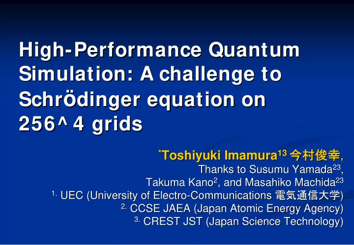
High- -Performance Quantum Performance Quantum High Simulation: A challenge to Simulation: A challenge to dinger equation on Schr dinger equation on Schr 256^ 4 grids 256^ 4 grids , * Toshiyuki Imamura 13 *
High- -Performance Quantum Performance Quantum High Simulation: A challenge to Simulation: A challenge to ö dinger equation on Schr ö dinger equation on Schr 256^ 4 grids 256^ 4 grids 今村俊幸 , * Toshiyuki Imamura 13 今村俊幸 * Toshiyuki Imamura 13 , 23 , Thanks to Susumu Yamada 23 , Thanks to Susumu Yamada 2 , and Masahiko Machida 23 Takuma Kano 2 , and Masahiko Machida 23 Takuma Kano 電気通信大学 ) Communications 電気通信大学 1. 1. UEC (University of Electro UEC (University of Electro- -Communications ) 2. CCSE JAEA (Japan Atomic Energy Agency) 2. CCSE JAEA (Japan Atomic Energy Agency) 3. CREST JST (Japan Science Technology) 3. CREST JST (Japan Science Technology)
� Outline □ Outline Physics, Review of Quantum Physics, Review of Quantum I . I . Simulation Simulation Mathematics, Numerical Algorithm Mathematics, Numerical Algorithm I I . I I . Grand Challenge, Parallel Computing I I I . Grand Challenge, Parallel Computing I I I . on ES on ES Numerical Results Numerical Results I V. I V. Conclusion Conclusion V. V. RANMEP2008, NCTS, Taiwan (清華大学 新竹 台湾) Jan. 4-8, 2008 2
I . Physics, I . Physics, Review of Quantum Review of Quantum Simulation, etc. Simulation, etc.
� □ 1.1, Quantum Simulation (1/ 2) (1/ 2) W W ’ down- -sizing sizing down S I S Crossover from Classical to Quantum ??? Crossover from Classical to Quantum ??? Classical Equation of Motion Classical Equation of Motion Schroedinger Equation Schroedinger Equation RANMEP2008, NCTS, Taiwan (清華大学 新竹 台湾) Jan. 4-8, 2008 4
� □ 1.2, Quantum Simulation (2/ 2) Numerical Simulation for Coupled Schrodinger Eq. Numerical Simulation for Coupled Schrodinger Eq. β: : ∝ 1 / W β 1/Mass ∝ 1 / W 1/Mass Ψ : possible state H β: : ∝ 1 / W β 1/Mass ∝ 1 / W 1/Mass not a value α: : α Coupling Coupling but a vector! Numerical method to solve the above equation Numerical method to solve the above equation : Spectral expansion by {u n } eigenvecs. Requirement of Exact Diagonalization Diagonalization for the Hamiltonian for the Hamiltonian Requirement of Exact RANMEP2008, NCTS, Taiwan (清華大学 新竹 台湾) Jan. 4-8, 2008 5
I I . Mathematics, I I . Mathematics, Numerical Algorithm, etc. Numerical Algorithm, etc.
� 2.1 □ 2.1 Krylov Krylov Subspace I teration Subspace I teration � Lanczos Lanczos (Traditional method) � (Traditional method) � Krylov+ GS Krylov+ GS : Simple, but : Simple, but shift+ invert shift+ invert version is needed version is needed � � LOBPCG LOBPCG (Locally Optimal Block PCG) � (Locally Optimal Block PCG) � { { Krylov Krylov base, Ritz vector, prior vector} : CG approach base, Ritz vector, prior vector} : CG approach � * * Restart at every iteration* * * * Restart at every iteration* * * * I NVERSE- -free* * free* * - -> Less Communication > Less Communication * * I NVERSE � Lanczos � LOBPCG RANMEP2008, NCTS, Taiwan (清華大学 新竹 台湾) Jan. 4-8, 2008 7
� 2.2 LOBPCG □ 2.2 LOBPCG � Costly! Since the block is updated at every Costly! Since the block is updated at every � iteration, MV operation is also required!! iteration, MV operation is also required!! Other Difficulties in implementation Other Difficulties in implementation • Breakdown of linear independency Breakdown of linear independency make our own DSYGV using LDL and deflation (not Cholesky Cholesky) ) make our own DSYGV using LDL and deflation (not • Growth of numerical error in {W,X,P} Growth of numerical error in {W,X,P} • detect numerical error and recalculate them automatically detect numerical error and recalculate them automatically 3*MV / every iteration • Choice of the shift • Choice of the shift 1*MV / every iteration • Portability Portability • RANMEP2008, NCTS, Taiwan (清華大学 新竹 台湾) Jan. 4-8, 2008 8
� 2.3 Preconditioning □ 2.3 Preconditioning -1 1 T~ H - � T~ H � H= A+ B 1 + B 2 + B 3 + B 4 + C 12 + C 23 + C 34 H= A+ B 1 + B 2 + B 3 + B 4 + C 12 + C 23 + C 34 100 H~A H~A No preconditioner H 1 (Point Jacobi) 10 H 2 (LDL) H~(A+B 1 ) H~(A+B 1 ) 1 H 3 (LDL) 0.1 Residual error -1 1 (A+B )A - H~ (A+B 1 (A+B 2 ) H~ (A+B 1 )A 2 ) 0.01 1e-3 Here, 1e-4 A: diagonal A+B x : block-tridiagonal 1e-5 � shift + LDL t is used 1e-6 0 100 200 300 400 500 Iteration count RANMEP2008, NCTS, Taiwan (清華大学 新竹 台湾) Jan. 4-8, 2008 9
I I I . Grand challenge, I I I . Grand challenge, Parallel Computing on ES, Parallel Computing on ES, etc. etc.
� 3.2 Technical I ssues on the Earth □ 3.2 Technical I ssues on the Earth Simulator Simulator � Programming model Programming model � � hybrid of distributed parallelism and thread � hybrid of distributed parallelism and thread parallelism. parallelism. Inter-Node 3-level parallelism Intra-Node • Inter Inter- -Node Node : : • node node node MPI (Message Passing Interface) (Message Passing Interface) MPI Low latency (6.63[us]) Low latency (6.63[us]) Processor 0 Very fast (11.63[GB/s]) Very fast (11.63[GB/s]) Processor 1 • Intra Intra- -Node Node : : • Vector processing Auto- -parallelization parallelization Auto Processor 7 OpenMP (thread (thread- -level parallelism) level parallelism) OpenMP • Vector Processor (most Vector Processor (most- -inner loops) : inner loops) : • Auto- -/manual /manual- - Vectorization Vectorization Auto RANMEP2008, NCTS, Taiwan (清華大学 新竹 台湾) Jan. 4-8, 2008 11
� 3.3 Quantum Simulation parallel code □ 3.3 Quantum Simulation parallel code � Application flow chart Application flow chart � Parallel LOBPCG solver Eigenmode developed on ES calculation Parallel code on ES Time Integrator Quantum state Parallel code on ES analyzer Visualized by AVS Visualization RANMEP2008, NCTS, Taiwan (清華大学 新竹 台湾) Jan. 4-8, 2008 12
� 3.4 Handling of Huge Data □ 3.4 Handling of Huge Data � Data distribution in case of a 4D array Data distribution in case of a 4D array � 2-dimensionnal loop 1-dimension loop ( k,l ) ( j ) decomposition decomposition N P / ) j / M P l , k i ( j l loop length=256 N P / i, j ) vector processing l , k i ( k intra-node parallelization N P : Number of MPI processes M P : Number of microtasking processes (=8) RANMEP2008, NCTS, Taiwan (清華大学 新竹 台湾) Jan. 4-8, 2008 13
� 3.5 Parallel LOBPCG □ 3.5 Parallel LOBPCG � Core implementation is MATRIX Core implementation is MATRIX- -VECTOR VECTOR mult mult. . � � 3 3- -level parallelism is carefully done in our implementation. level parallelism is carefully done in our implementation. � � In Inter In Inter- -node parallelization, communication pipelining is used. node parallelization, communication pipelining is used. � � In the Rayleigh In the Rayleigh- -Ritz part, SCALAPACK is used. Ritz part, SCALAPACK is used. � do l=1,256 :: inter inter- -node parallelism node parallelism do k=1,256 :: inter inter- -node parallelism node parallelism do j=1,256 :: intra intra- -node (thread) parallelism node (thread) parallelism � LOBPCG do i=1,256 :: vectorization vectorization w(i,j,k,l)=a(i,j,k,l)*v(i,j,k,l) & +b*(v(i+1,j,k,l)+・・・) +c*(v(i+1,j+1,k,l)+・・・) enddo enddo enddo enddo Acg.f Acg.f RANMEP2008, NCTS, Taiwan (清華大学 新竹 台湾) Jan. 4-8, 2008 14
I V. Numerical Results, I V. Numerical Results,
� 4.1, Numerical Result □ � Preliminary test of our Preliminary test of our eigensolver eigensolver � � 4 4- -junction system: junction system: - -> 256^ 4 dimension > 256^ 4 dimension � Convergence history 1e+4 the ground state Performance the 2nd lowest state 1e+2 the 3rd lowest state the 4th lowest state the 5th lowest state CPUs time[s] ] TFLOPS CPUs time[s TFLOPS 1 the 6th lowest state Residual error the 7th lowest state the 8th lowest state 2048 3118 3.65 2048 3118 3.65 1e-2 the 9th lowest state the 10th lowest state 1e-4 3072 2535 4.49 3072 2535 4.49 1e-6 4096 1621 7.02 4096 1621 7.02 1e-8 (5 eigenmodes) 1e-10 1e-12 0 500 1000 1500 2000 2500 3000 Iteration count (10 eigenmodes) RANMEP2008, NCTS, Taiwan (清華大学 新竹 台湾) Jan. 4-8, 2008 16
� □ 4.2, Numerical Result (Scenario) Question: Synchronization or I ndependence (Localization) Question: Synchronization or I ndependence (Localization) The Simplest Case: (two Junctions) The Simplest Case: (two Junctions) Capacitive Capacitive Coupling Coupling ? ? Potential Change: Potential Change: Initial State Initial State Only a Single Junction Only a Single Junction RANMEP2008, NCTS, Taiwan (清華大学 新竹 台湾) Jan. 4-8, 2008 17
� □ 4.3, Numerical Result Two- -Stacked Intrinsic Josephson Junction Stacked Intrinsic Josephson Junction Two θ 2 Classical Regime: Classical Regime: Independent Dynamics Independent Dynamics Quantum Regime: Quantum Regime: ? ? θ 1 RANMEP2008, NCTS, Taiwan (清華大学 新竹 台湾) Jan. 4-8, 2008 18
� □ α α= = 0.4 0.4 β= β = 0.2 0.2 q 1 q 1 q 2 q 2 t=0.0(a.u.) t=2.9(a.u.) q 1 q 1 q 2 q 2 RANMEP2008, NCTS, Taiwan (清華大学 新竹 台湾) Jan. 4-8, 2008 19 t=9.2(a.u.) t=10.0(a.u.)
Recommend
More recommend
Explore More Topics
Stay informed with curated content and fresh updates.
