SELECT THE RIGHT ABSTRACT INTERESTINGNESS MEASURE FOR ASSOCIATION - PowerPoint PPT Presentation

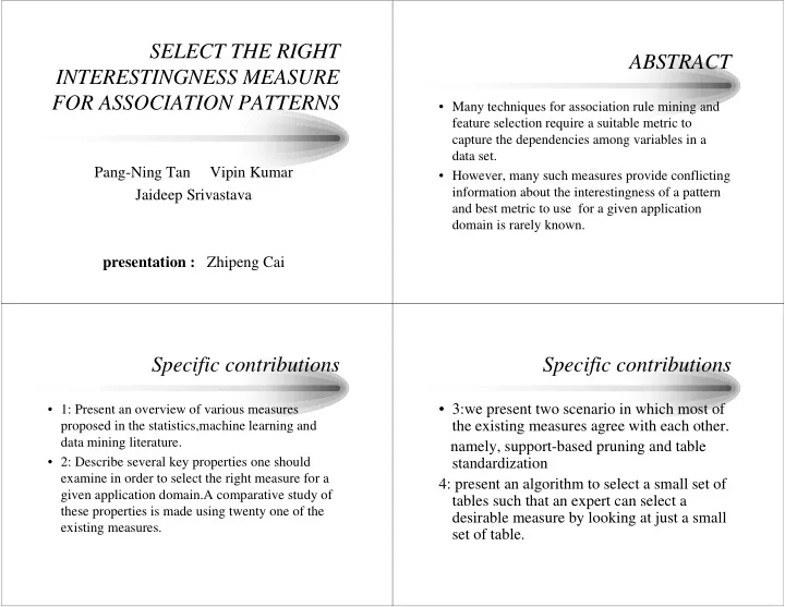
SELECT THE RIGHT ABSTRACT INTERESTINGNESS MEASURE FOR ASSOCIATION PATTERNS • Many techniques for association rule mining and feature selection require a suitable metric to capture the dependencies among variables in a data set. Pang-Ning Tan Vipin Kumar • However, many such measures provide conflicting information about the interestingness of a pattern Jaideep Srivastava and best metric to use for a given application domain is rarely known. presentation : Zhipeng Cai Specific contributions Specific contributions • 3:we present two scenario in which most of • 1: Present an overview of various measures the existing measures agree with each other. proposed in the statistics,machine learning and data mining literature. namely, support-based pruning and table • 2: Describe several key properties one should standardization examine in order to select the right measure for a 4: present an algorithm to select a small set of given application domain.A comparative study of tables such that an expert can select a these properties is made using twenty one of the desirable measure by looking at just a small existing measures. set of table.

Table1:A 2*2 contingency table INTRODUCTION for variables A and B • The central task of association rule mining is to find sets of binary variables that co-occur together B B frequently in a transaction database. f 11 • Analysis often requires a suitable metric to capture A f f f + 11 10 1 the dependencies among variables. • These metrics are defined in terms of the f f f A + 01 00 0 frequency counts tabulated in a 2*2 contingency table. f f + + 1 0 Table 3:Ranking of contingency table using various interestingness measures Table 2:Example of contingency tables

Interestingness Measures for Association Patterns Interestingness Measures for Association Patterns Interestingness Measures for Association Patterns Two situation Preliminaries • T(D)={t1,t2,t3….t n} denote the set of patterns . • 1: the measures may become highly correlated when support-based pruning is • P is the set of measures available to an analyst. M ∈ used. • P ∈ ∈ ∈ ∈ • M(T)={m1,m2,m3….m n},which corresponds to • 2: after standardizing the contingency tables the values of M for each contingency table that to have uniform margins, many of the well- belongs to T(D). known measures become equivalent each • M(T) can also be transformed into a ranking other. vector Om(T)={O1,O2,….On}.

Desired properties of a measure Definition 1: three key properties • P1: M=0 if A and B are statistically • [Similarity between measures] independent; • Two measures of association, M1 and M2, are • P2: M monotonically increases with similar to each other with respect to the data set D P(A,B)when P(A) and P(B) remain the if the correlation between Om1(T) and Om2(T) same. is greater than or equal to some positive threshold • P3: M monotonically decreases with t. P(A)(or P(B)) when the rest of the parameters (P(A,B) and P(B) or P(A)) remain unchanged. • Property 2:[Row/Column scaling invariance] • Let R=C=[k1 0 ;0 k2] be a 2*2 square Other properties of a measure matrix. • A measure O is invariant under row and • Property 1: [symmetry under variable column scaling if O(RM)=O(M) and permutation] O(MC)=O(M) for all contingency • A measure O is symmetric under variable matrices,M T = permutation, A B,if for all O ( M ) O ( M ) contingency matrices M

Property 3: Antisymmetry under Row/Column permutation . Property 4: Inversion Invariance • Let S=[0 1; 1 0] be a 2*2 permutation matrix. A normalized measure O is antisymmetric under the row permutation operation. • Let S=[0 1;1 0] be a 2*2 permutation • O(SM)= - O (M). matrix . A measure O is invariant under the • Under the column permutation operation inversion operation , if O(SMS)=O(M) for • O(MS)=-O(M) all contingency matrices M. • Property 5: Null Invariance Table 6 properties of interestingness measures • A binary measure of association is null- invariant if O(M+C)=O(M) where C=[0 0; 0 k] and is a positive constant.

Summary Table 6 properties of interestingness measures • where: P1: O(M) = 0 if det(M) = 0, i.e. , whenever A and B are • The discussion in this section suggests that statistically independent. there is no measure that is better than others • P2: O(M2) > O(M1) if M2 = M1+ [k –k;-k k] • P3: O(M2) < O(M1) if M2=M1+ [0 k;0 -k] or M2=M1+ [0 0;k -k] . in all application domains . • O1: Property1: symmetry under variable permutation O2: Property2: Row/Column scaling invariance • • Thus, in order to find the right measure, one • O3: Property3: Antisymmetry under Row/Column permutation. must match the desired properties of an • O3’:Property4: inversion invariance. • O4:: Property5: Null invariance application against the properties of the • Yes*: yes if measure is normalized. existing measures. • No*:Symmetry under row or column permulation. • No**:No unless the measure is symmetrized by taking max(M(A,B),M(B,A)). Equivalence of measures under support constraints Effect of support-based pruning • Support is a widely-used measure in association rule mining because it represents the statistical significance of a pattern. • We now describe two additional consequences of using the support measure. 1: Equivalence of measures under support constraints. 2: Elimination of poorly correlated tables using support-based pruning.

Elimination of poorly correlated tables using support-based pruning. TABLE STANDARDIZATION • Standardization is a widely-used technique. • standardization is needed to get a better idea of the underlying association between * = = = = * = = = = * = = = = * = = = = f * * * f * * * f * * * f * * * N / 2 f f f f f f f f f f f f N N N / / / 2 2 2 + + + + + + + + + + + + + + + + 1 1 1 1 0 0 0 0 1 1 1 1 0 0 0 0 marginals are variables by transforming an existing table so that their equal. = = = = * * * * f f f f N / 2 + + + + 1 0 1 0 * f • Row scaling: = − × + ( k ) ( k 1 ) i f f Table 7: Table Standardization ij ij ( k ) f + j * f + = × + ( k 1 ) ( k ) j f f • Column scaling: ij ij ( k ) f + j * f + + ( k 1 ) = ( k ) × j f f ij ij ( k ) f + j

Table 8:Rankings of contingency Three equation for fix the table after IPF standardization standardized table = * * f f • 1 11 00 = * * f f • 2 10 01 + = * * f f N / 2 • 3 11 10 Measure Selection Based on Example bankings by experts P ( A , B ) P ( A , B ) • Odds ratio : • 1:Random :randomly select k out of the P ( A , B ) P ( A , B ) overall N tables and present them to the * * experts. f f f f = 11 00 11 00 Fourth equations: * * f f f f 10 01 10 01 • 2:Disjoint: select k tables that are “furthest” N f f Apart according to their average ranking = = * * 11 00 f f 11 00 + 2 ( f f f f ) and would produce the largest amount of 11 00 10 01 ranking conflicts. N f f = = 10 01 * * f f 10 01 + 2 ( f f f f ) 11 00 10 01

= − D ( S , S ) max S ( i , j ) S ( i , j ) s , T T s , i , j = − D ( S , S ) max S ( i , j ) S ( i , j ) s , T T s , i , j Conclusions • 1:Describe several key properties. • 2:There are situations in which many of these measure that is consistently with each other • 3:Present an algorithm to select a small set of tables that an expert can find the most appropriate measure by looking at this small set of table.