Maximum Entropy & Subjective Interestingness Jill illes V s - PowerPoint PPT Presentation
Maximum Entropy & Subjective Interestingness Jill illes V s Vreeken 26 June une 2015 2015 Questions of the day How can we find things that are interesting with regard to what we already know ? How can we measure subjective
Maximum Entropy & Subjective Interestingness Jill illes V s Vreeken 26 June une 2015 2015
Questions of the day How can we find things that are interesting with regard to what we already know ? How can we measure subjective interestingness ?
What is interesting? something that increa ease ses our knowledge about the data
What is a good result? something that red educ uces our uncertainty about the data (ie. increases the likelihood of the data)
What is really good? something that, in simpl ple term rms, st strongly r red educ uces our uncertainty about the data (maximise likelihood, but avoid overfitting)
Let’s make this visual universe of possible datasets our dataset D
dimensions, margins Given what we know possible datasets, given current knowledge all possible our dataset D datasets
dimensions, margins, More knowledge... pattern P 1 all possible our dataset D datasets
dimensions, margins, Fewer possibilities... patterns P 1 and P 2 all possible our dataset D datasets
dimensions, margins, Less uncertainty. the key structure all possible our dataset D datasets
dimensions, margins, Maximising certainty patterns P 1 and P 2 knowledge added by P 2 all possible our dataset D datasets
How can we define ‘uncertainty’ and ‘simplicity’? interpr rpreta tability ty and informativen eness ess are intrinsically subjective
Measuring Uncertainty We need access to the likelihood ood of data D given background knowledge B 𝑞 ( 𝐸 ∣ 𝐶 ) such that we can calculate the gain for X − 𝑞 ( 𝐸 ∣ 𝐶 ) 𝑞 𝐸 𝐶 ∪ 𝑌 …which distribution should we use?
Measuring Surprise We need access to the likelihood of result X given background knowledge B 𝑞 ( 𝑌 ∣ 𝐶 ) such that we can mine the data for X that have a low likelihood, that are surp rpris rising …which distribution should we use?
Approach 2: Maximum Entropy ‘the best distribution 𝑞 ∗ satisfies the background knowledge, but makes no further assumptions’ (Jaynes 1957; De Bie 2009)
Approach 2: Maximum Entropy ‘the best distribution 𝑞 ∗ sati satisfies th the bac ackgr ground knowledge dge, but makes no further assumptions’ in other words, 𝑞 ∗ assigns the correct probability mass to the background knowledge instances: 𝑞 ∗ is a maximum likelihood estimator (Jaynes 1957; De Bie 2009)
Approach 2: Maximum Entropy ‘the best distribution 𝑞 ∗ satisfies the background knowledge, but ma makes no no fur urthe her a assum umption ons’ in other words, 𝑞 ∗ spreads probability mass around as evenly as possible: 𝑞 ∗ does not have any specific bias (Jaynes 1957; De Bie 2009)
Approach 2: Maximum Entropy ‘the best distribution 𝑞 ∗ satisfies the background knowledge, but makes no further assumptions’ ver ery usef useful for data mining: unbiased sed measurement of subject ective e interest estingness ness (Jaynes 1957; De Bie 2009)
Constraints and Distributions Let 𝐶 be our set of constraints 𝑜 } 𝐶 = { 𝑔 1 , … , 𝑔 Let 𝐷 be the set of admissible distributions 𝑗 ∈ 𝐶 } 𝐷 = 𝑞 ∈ 𝐐 𝑞 𝑔 𝑗 = 𝑞 � 𝑔 𝑗 for 𝑔 We need the most uni unifor ormly distributed 𝑞 ∈ 𝐐
Uniformity and Entropy Uniformity ↔ Entropy 𝐼 𝑞 = − � 𝑞 ( 𝑌 = 𝑦 )log 𝑞 ( 𝑌 = 𝑦 ) 𝑦∈𝐘 tells us the ent ntrop opy of a (discrete) distribution 𝑞
Maximum Entropy We want access to the distribution 𝑞 ∗ with maximum mum entro ropy ∗ = argmax 𝑞∈𝐷 𝐼 ( 𝑞 ) 𝑞 𝐶 better known as the ma maximum um e ent ntropy mod model for constraints set 𝐶
Maximum Entropy We want access to the distribution 𝑞 ∗ with maximum mum entro ropy ∗ = argmax 𝑞∈𝐷 𝐼 ( 𝑞 ) It can be shown that 𝑞 ∗ is well defined 𝑞 𝐶 there always exist a unique 𝑞 ∗ with maximum entropy for any constrained set 𝐷 better known as the ma maximum um e ent ntropy mod model for constraints set 𝐶 (that’s not completely true, some esoteric exceptions exist)
Does this make sense? Any distribution with less-than-maximal entropy must have a reaso ason for this. Less entropy means not-as-uniform-as-possible, that is, undue peaks of probability mass. That is, reduced entropy = late tent assu assumptions, exactly what we want to avoid!
Optimal-worst-case Recall that through Kraft’s inequality probab ability ty di distr stribution ↔ enco codin ing The MaxEnt distribution for 𝐶 gives the mi mini nimu mum worst-case expected encoded length over an any y distribution that satisfies this background knowledge.
Some examples Mean and interval? uniform variance? Gaussian positive? exponential discrete? geometric … But… what about distributions for like data, patterns, and stuff?
MaxEnt Theory To use MaxEnt, we need theo heory y for modelling data given background knowledge Patterns itemset frequencies (Tatti ’06, Mampaey et al. ’11) Real-valued Data Binary Data margins (De Bie ‘09) margins (Kontonasios et al. ‘11) sets of cells (Kontonasios et al. ‘13) tiles (Tatti & Vreeken, ‘12)
Finding the MaxEnt distribution You can finding the MaxEnt distribution by solving the following system of linear constraints max − � 𝑞 𝑦 log 𝑞 ( 𝑦 ) 𝑞 ( 𝑦 ) 𝑦 𝑡 . 𝑢 . � 𝑞 𝑦 𝑔 𝑗 𝑦 = 𝛽 𝑗 for all 𝑗 𝑦 � 𝑞 𝑦 = 1 𝑦 * for discrete data
Exponential Form Let 𝑞 be a probability density satisfying the constraints for 1 ≤ 𝑗 ≤ 𝑛 �𝑞 𝑦 𝑔 𝑗 𝑦 𝑒𝑦 = 𝛽 𝑗 𝑇 then we can write the MaxEnt distribution as 𝑞 ∗ = 𝑞 𝜇 𝑦 ∝ � exp 𝜇 0 + � 𝜇 𝑗 𝑔 𝑗 𝑦 𝐸 ∉ 𝒶 𝑔 𝑗 ∈𝐶 0 𝐸 ∈ 𝒶 where we choose the lambdas, Lagrange multipliers, to satisfy the constraints, and where 𝒶 is a collection of databases s.t. 𝑞 ( 𝐸 ) = 0 for all 𝑞 ∈ 𝒬 (Csizar 1975)
Solving the MaxEnt The Lagrangian is 𝑀 𝑞 𝑦 , 𝜈 , 𝜇 = − � 𝑞 𝑦 log 𝑞 𝑦 + � 𝜇 𝑗 � 𝑞 𝑦 𝑔 𝑗 𝑦 − 𝛽 𝑗 + 𝜈 � 𝑞 𝑦 − 1 𝑦 𝑗 𝑗 𝑦 We set the derivative w.r.t. 𝑞 𝑦 to 0 and get 𝑞 𝑦 = 1/ 𝑎 𝜇 exp � 𝜇 𝑗 𝑔 𝑗 𝑦 𝑗 where 𝑎 𝜇 = ∑ exp is called the partitio ion n func nction ( ∑ 𝜇 𝑗 𝑔 𝑗 ( 𝑦 )) 𝑦 𝑗
En Garde! We may substitute 𝑞 ( 𝑦 ) in the Lagrangian to obtain the dua ual obje ject ctiv ive 𝑀 𝜇 = log 𝑎 𝜇 − � 𝜇 𝑗 𝛽 𝑗 𝑗 Minimizing the dual gives the maximal solution to the original problem. Moreover, it is conve vex. x.
Inferring the Model The problem is convex means we can use an any y convex optimization strategy. Standard approaches include iterative scaling, gradient descent, conjugate gradient descent, Newton’s method, etc.
Inferring the Model Optimization requires calculating p for datasets and tiles this is easy asy for itemsets and frequencies, however, this is PP PP-hard rd
MaxEnt for Binary Databases Constraints: the expec ected ed row and column margins 𝑛 � 𝑞 𝐸 � 𝑒 𝑗𝑗 = 𝑠 𝑗 𝐸∈ 0 , 1 𝑜 × 𝑛 𝑗=1 𝑜 � 𝑞 𝐸 � 𝑒 𝑗𝑗 = 𝑑 𝑗 𝐸∈ 0 , 1 𝑜 × 𝑛 𝑗=1 (De Bie 2010)
MaxEnt for Binary Databases Using the Lagrangian, we can solve 𝑞 𝐸 1 𝑠 + 𝜇 𝑗 𝑑 𝑞 𝐸 = � 𝑑 exp 𝑒 𝑗𝑗 𝜇 𝑗 𝑠 , 𝜇 𝑗 𝑎 𝜇 𝑗 𝑗 , 𝑗 where 𝑑 = 𝑠 + 𝜇 𝑗 𝑠 , 𝜇 𝑗 𝑑 𝑎 𝜇 𝑗 � exp 𝑒 𝑗𝑗 𝜇 𝑗 𝑒 𝑗𝑗 ∈ { 0 , 1 }
MaxEnt for Binary Databases Using the Lagrangian, we can solve 𝑞 𝐸 1 𝑠 + 𝜇 𝑗 𝑑 𝑞 𝐸 = � 𝑑 exp 𝑒 𝑗𝑗 𝜇 𝑗 𝑠 , 𝜇 𝑗 𝑎 𝜇 𝑗 𝑗 , 𝑗 Hey! 𝑞 𝐸 is a product of independent elements! That’s handy! We did id not enforce this property, it’s a consequence of MaxEnt. Following, every element is hence Bernoulli distributed, 𝑠 +𝜇 𝑗 𝑑 𝜇 𝑗 with a success probability of exp 𝑑 𝑠 +𝜇 𝑗 1+exp 𝜇 𝑗
What have you done for me lately? Okay, say we have this 𝑞 ∗ , what is it useful for? Given 𝑞 ∗ we can sample data from 𝑞 ∗ , and compute empirical p-values (just like with swap randomization) compute the likelihood of the observed data, and compute how surprising our findings are given 𝑞 ∗ , and compute exact p-values
Expected vs. Actual Swap randomization and MaxEnt can both maintain margins. MaxEnt constrains the expec ected ed margins. Swap randomization constrains the act ctual l margins. Does this matter?
MaxEnt Theory To use MaxEnt, we need theo heory y for modelling data given background knowledge Binary Data Real-valued Data margins (De Bie, ‘09) margins (Kontonasios et al. ‘11) tiles (Tatti & Vreeken, ‘12) arbitrary sets of cells (now) allow for ite terative ve mining
MaxEnt for Real-Valued Data Current state of the art can incorporate means, ns, variance, and higher order moments, as well as histog ogram am information over arbitra trary sets of cells (Kontonasios et al. 2013)
Recommend
More recommend
Explore More Topics
Stay informed with curated content and fresh updates.
