Scientific Computing with Fortran 95 (4EV04) dr.ir. Martien A. - PowerPoint PPT Presentation
Scientific Computing with Fortran 95 (4EV04) dr.ir. Martien A. Hulsen m.a.hulsen@tue.nl dr.ir. Patrick D. Anderson p.d.anderson@tue.nl Website: http://www.mate.tue.nl/~hulsen under link Scientific Computing with Fortran 95.
Scientific Computing with Fortran 95 (4EV04) dr.ir. Martien A. Hulsen m.a.hulsen@tue.nl dr.ir. Patrick D. Anderson p.d.anderson@tue.nl Website: http://www.mate.tue.nl/~hulsen under link ‘Scientific Computing with Fortran 95’. – Scientific Computing with Fortran 95 (4EV04) / Section Materials Technology (MaTe) –
Goals ⊲ to learn the basic elements of Fortran 95. ⊲ to enter the fascinating world of scientific computing by solving a scientific problem: find the critical parameters where the fiber spinning process becomes linearly unstable. NOTE: this is project B.
Why Fortran in the 21 st century? Walt Brainerd (2003): “Fortran is still the best programming language for numerical/scientific computing”. Reasons include: ⊲ designed for speed ⊲ portability (Windows laptop ⇔ 1024-processor supercomputer) ⊲ millions of lines of existing and well tested codes ⊲ more straightforward to learn and use than most “modern” languages ⊲ designed for and by numerical/scientific professionals
Fortran programming language ⊲ First version developed in the period 1954-1957 at IBM ⊲ First standard: Fortran 66 ⊲ ‘Old style’ standard: Fortran 77 ⊲ New modern standards: Fortran 90, Fortran 95 – array syntax (whole array operations, dynamic memory allocation, ...) – modules (modular programming, data hiding and abstract data types, module procedures, interfaces and operators, global data)
Fortran programming language: new developments ⊲ Latest revision, approved by ISO in 2004: Fortran 2003 – object oriented programming – handling of floating point exceptions – interoperability with C ⊲ Draft standard: Fortran 2008 – coarrays
Learning Fortran 95 ⊲ Book: S.J. Chapman: “Fortran 90/95 for Scientists and Engineers” (2004) ⊲ Study guide for the book on our website (first nine chapters). ⊲ Sources of all examples in the book available online (see website) ⊲ Compiler for Windows: Silverfrost FTN95 with Plato IDE (campus licence, see our website). ⊲ FAQ on website
Fiber spinning A 0 A(z) z �✁�✁�✁�✁� ✂✁✂✁✂✁✂✁✂ v(z) v D r 0 ☎✁☎✁☎✁☎✁☎ ✄✁✄✁✄✁✄✁✄ v 0 ✄✁✄✁✄✁✄✁✄ ☎✁☎✁☎✁☎✁☎ L ⊲ include inertia Re � = 0 ⊲ steady state A = ¯ A ( z ) , v z = ¯ v z ( z ) : analytical solution
Draw resonance
Linear stability analysis Decompose with A ′ and v ′ z small: A ( z, t ) = ¯ A ( z ) + A ′ ( z, t ) v z ( z ) + v ′ v z ( z, t ) = ¯ z ( z, t ) Assume: ∞ A ′ = e λ j t ˆ � A j ( z ) j =1 ∞ � e λ j t ˆ v ′ z = v j ( z ) j =1 Unstable: Re( λ j ) > 0 for some j .
Numerical solution: matrix eigenvalue problem Finite difference approximation leads to = S or ( S ¯ ) u = 0 λu ¯ u ¯ − λI ˜ ˜ ˜ ˜ Notes: ⊲ Can be solved with LAPACK or NAG library routines. ⊲ Study dependance on the Reynolds number of the critical D r . ⊲ Special case Re = 0 .
Work plan and finalization ⊲ Suggested work plan on website. ⊲ Theoretical background (with all equations) on website. ⊲ Finalization: a working, nicely structured Fortran 95 code + a short presentation. ⊲ Everything should be finished on Tuesday 9/6.
Final advise Have fun
Recommend
More recommend
Explore More Topics
Stay informed with curated content and fresh updates.
