Getting started with Fortran branches loops 1 2 Why learn - PowerPoint PPT Presentation

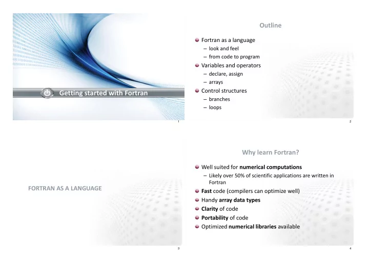
Outline Fortran as a language – look and feel – from code to program Variables and operators – declare, assign – arrays Control structures Getting started with Fortran – branches – loops 1 2 Why learn Fortran? Well suited for numerical computations – Likely over 50% of scientific applications are written in Fortran FORTRAN AS A LANGUAGE Fast code (compilers can optimize well) Handy array data types Clarity of code Portability of code Optimized numerical libraries available 3 4

Short history of Fortran Short history of Fortran John W. Backus et al (1954): The IBM Mathematical Fortran 2003 (2004): a major revision, adding e.g. object- For mula Tran slating System oriented features, C-bindings – ”Fortran 95/2003” is the current de facto standard Early years development: Fortran II (1958), Fortran IV (1961), Fortran 66 & Basic Fortran (1966) The latest standard is Fortran 2008 (2010): a minor Fortran 77 (1978) revision Fortran 90 (1991) a major revision and Fortran 95 (1997) – Most notable addition: Fortran coarray syntax a minor revision to it – Compiler support nearly complete – The next revision: Fortran 2015 5 6 Compiling and linking Transition from code to a program Compile and link in one go, execute the binary source code (.f, .F, .f90, .F90) gfortran main.f90 -o foo ./foo INCLUDE In more complex cases (multiple sources) compiler output files compiler – Compile each source code file (.f90) into an object file (.o) (optional) modules gfortran -c main.f90 object code gfortran -c sub.f90 (.o, .so) – Link object files into a binary and execute the binary libraries linker output gfortran -o foo main.o sub.o linker (.a, .so) (optional) ./foo # after some modifications in “sub.f90” executable gfortran – c sub.f90 gfortran -o foo main.o sub.o ./foo 7 8

Look and feel Source code remarks program square_root_example Free format source code, but ! comments start with an exclamation point. – A variable name can be no longer than 31 characters containing ! you will find data type declarations, couple arithmetic operations ! and an interface that will ask a value for these computations. only letters, digits or underscore, and must start with a letter implicit none real :: x, y – Maximum row length is 132 characters intrinsic sqrt ! fortran standard provides many commonly used functions No distinction between lower and uppercase characters ! command line interface. ask a number and read it in – Character strings are case sensitive write (*,*) 'give a value (number) for x:' read (*,*) x Line break is the statement separator y = x**2+1 ! power function and addition arithmetic – If a line is ended with an ampersand (&), the line continues onto write (*,*) 'given value for x:', x the next line (max. 39 continuation lines allowed) write (*,*) 'computed value of x**2 + 1:', y – Semicolon (;) is the separator between statements on a single ! print the square root of the argument y to screen write (*,*) 'computed value of sqrt(x**2 + 1):', sqrt(y) line end program square_root_example 9 10 Variables Variables must be declared at the integer :: n0 beginning of the program or procedure where they are used real :: a, b real :: r1=0.0 the intrinsic data types in Fortran are VARIABLES integer , real , complex , character and complex :: c logical complex :: imag_number=(0.1, 1.0) They can also be given a value at character(len=80) :: place declaration (not recommended) character(len=80) :: name='james bond' Constants are defined with the logical :: test0 = .true. PARAMETER clause – they cannot be logical :: test1 = .false. altered after their declaration real, parameter :: pi=3.14159 11 12

Operators Arrays Arithmetic operators real :: x,y integer, parameter :: m = 100, n = 500 integer :: i = 10 integer :: idx(m) x = 2.0**(-i) !power function and negation precedence: first real :: vector(0:n-1) x = x*real(i) !multiplication and type change precedence: second By default, Fortran indexing starts real :: matrix(m, n) x = x/2.0 !division precedence: second from 1 i = i+1 !addition precedence: third character (len=80) :: screen (24) i = i-1 !subtraction precedence: third Relational operators ! or < or .lt. !less than <= or .le. !less than or equal to integer, dimension(m) :: idx == or .eq. !equal to real, dimension(0:n-1) :: vector /= or .ne. !not equal to real, dimension(m, n) :: matrix > or .gt. !greater than character(len=80), dimension(24) :: screen >= or .ge. !greater than or equal to Logical operators .not. !logical negation precedence: first .and. !logical conjunction precedence: second .or. !logical inclusive disjunction precedence: third 13 14 Conditionals (if-else) Conditionals allow the program to execute different code based on some condition(s) if (condition) then CONTROL STRUCTURES ! do something else if (condition2) then ! .. or maybe alternative something else else ! .. or at least this end fi Condition can be anything from a simple comparison to a complex combination using logical operators 15 16

Conditionals example Loops 2 program placetest Three loop formats available in Fortran implicit none 1 logical :: in_square1, in_square2 – integer counter (fixed number of iterations) real :: x, y – condition controlled (do until condition is false) write (*,*) ’ give point coordinates x and y’ read (*,*) x, y – explicit exit statement in_square1 = (x >= 0. .and. x <= 2. .and. y >= 0. .and. y <= 2.) in_square2 = (x >= 1. .and. x <= 3. .and. y >= 1. .and. y <= 3.) if (in_square1 .and. in_square2) then ! inside both do {control clause} write (*,*) ’ point within both squares ’ ! execute something again and again until stopped else if (in_square1) then ! inside square 1 only end do write (*,*) ’ point inside square 1’ else if (in_square2) then ! inside square 2 only ! where the control clause (optional) is either of the form write (*,*) ’ point inside square 2’ ! i=init_value, max_value, increment else ! both are .false. ! or a condition to execute while true write (*,*) ’ point outside both squares ’ ! while (condition) end if end program placetest 17 18 Loops example Loops example integer :: i, stepsize, numberofpoints real :: x, totalsum, eps integer, parameter :: max_points=100000 totalsum = 0.0 real :: x_coodinate(max_points), x, totalsum ! do loop without loop control ! a do-loop with an integer counter (count controlled) do stepsize = 2 read(*,*) x do i = 1, max_points, stepsize if (x < 0) then x_coordinate(i) = i*stepsize*0.05 exit ! = exit the loop end do else if (x > upperlimit) then ! condition controlled loop (do while) cycle ! = do not execute any further statements, but totalsum = 0.0 ! instead cycle back to the beginning of the loop read(*,*) x end if do while (x > 0) totalsum = totalsum + x totalsum = totalsum + x read(*,*) x end do end do 19 20

Labels example Select case program gcd integer :: i select case statements ! computes the greatest common divisor, Euclidean algorithm logical :: is_prime, implicit none matches the entries of a test_prime_number integer :: m, n, t list against the case index write (*,*)’ give positive integers m and n :’ ... read(*,*) m, n – Only one found match is write (*,*)’m:’, m,’ n:’, n Labels can be given to select case (i) allowed positive_check: if (m > 0 .and. n > 0) then control structures and used case (2,3,5,7) main_algorithm: do while (n /= 0) – Usually arguments are is_prime = .true. in conjunction with e.g. exit t = mod(m,n) case (1,4,6,8:10) and cycle statements character strings or m = n is_prime = .false. n = t integers case default end do main_algorithm is_prime=test_prime_number(i) – default branch if no write (*,*) ’ greatest common divisor : ’,m end select else match found write (*,*) ’ negative value entered ’ ... end if positive_check end program gcd 21 22 Summary Fortran is – despite its long history – a modern programming language designed especially for scientific computing – Versatile, quite easy to learn, powerful In our first encounter, we discussed – Variables, data types, operators – Control structures: loops and conditionals 23

Outline Structured programming Modules Procedures: functions and subroutines Interfaces Procedure arguments Procedures and modules 24 25 Structured programming Modular programming Structured programming based on program sub-units Modularity means dividing a program into minimally ( functions , subroutines and modules ) enables dependent modules – Enables division of the program into smaller self-contained – Testing and debugging separately units – Re-use of code Fortran modules enable – Improved readability – Global definitions of procedures, variables and constants – Re-occurring tasks – Compilation-time error checking The key to success is in well defined data structures and – Hiding implementation details scoping, which lead to clean procedure interfaces – Grouping routines and data structures – Defining generic procedures and custom operators 26 27