Same-Decision Probability: A New Tool for Decision Making Suming - PowerPoint PPT Presentation
Same-Decision Probability: A New Tool for Decision Making Suming Chen Arthur Choi Adnan Darwiche UCLA Introduction Bayesian Network N We make a decision based on D . Example: D Health state of D a patient. Patient healthy: D
Same-Decision Probability: A New Tool for Decision Making Suming Chen Arthur Choi Adnan Darwiche UCLA
Introduction Bayesian Network N • We make a decision based on D . • Example: D – Health state of D a patient. • Patient healthy: D = True • Patient unhealthy: D = False
Introduction (2) Bayesian Network N D Tumor Test = True Diagnosis: Patient is sick.
Introduction (3) Bayesian Network N Test Reliable = False D Tumor Test = True Diagnosis: Patient is healthy
Stopping Criteria Bayesian Network N Gender Test Reliable = False D Facial Hair Tumor Test = True Diagnosis: Patient is healthy
Stopping Criteria (2) Bayesian Network N Radiation Test Reliable = False Exposure D High Fever Tumor Test = True Diagnosis: Patient is healthy
Selection Criteria Bayesian Network N Radiation H Exposure Which variables D should we observe? High Fever H Diagnosis: Patient is healthy
Decision Tools Current Decision Tools Stopping Criteria Selection Criteria • Expend budget for • Entropy reduction observation. • Margins of confidence • Pr( D=d | e ) ≥ T • Utility (influence • Value of information of diagram setting). observations > cost.
Decision Tools Current Decision Tools Stopping Criteria Selection Criteria • Expend budget for • Entropy reduction observation. • Margins of confidence • Pr( D=d | e ) ≥ T • Utility (influence • Value of information of diagram setting). observations > cost. New Decision Tools • Same-decision Probability • Same-decision Probability
Same-Decision Probability Same-Decision Probability - probability that we would have made the same decision had we known some additional variables. – Useful as a stopping criteria. – Useful as a selection criteria.
Same-Decision Probability Example • Naive Bayes Classifier with missing D features D =T 0.60 • E 1 = True D =F 0.40 • Two features, H 1 and H 2 unobserved. D • Pr(D=T| e ) = 0.778 H H E 1 H 1 H 2 D =T D =F * =T 0.70 0.30 * =T 0.30 0.70
Same-Decision Probability Example • Naive Bayes Classifier with missing D features D =T 0.60 • E 1 = True D =F 0.40 • Two features, H 1 and H 2 unobserved. D • Pr(D=T| e ) = 0.778 Pr(h|e) H 1 H 2 Pr(D=T|h,e) H H T T 0.401 0.95 E 1 H 1 H 2 T F 0.21 0.778 F T 0.21 0.778 F F 0.179 0.39 D =T D =F SDP is calculated to be 0.401 + 0.21 * =T 0.70 0.30 * =T 0.30 0.70 + 0.21 = 0.821.
Same-Decision Probability Definition The SDP over variables H, with a decision function F , interest variable D , and evidence e , is defined as: SDP( F, D, H , e ) = h [ F (Pr( D | h , e ))] h Pr( h | e ) [.] h – indicator function – 1 when F(Pr ( D | h , e )) = F(Pr ( D | e )) – 0 otherwise
SDP – Stopping Criteria • Calculating SDP can act as a stopping criteria. – Provides a quantitative measure of how likely our decision is to change if some unobserved variables were known. – Can tell us when no other further observations are necessary.
SDP – Stopping Criteria Example Threshold-based decision: D Pr( D =+| e ) ≥ 0.55 D = + D = - D = + D = - S 1 S 2 S 3 S 4 S 1 = + 0.55 0.45 S 2 = + 0.55 0.45 S 1 = - 0.45 0.55 S 2 = - 0.45 0.55 D D = + D = - D = + D = - D =+ 0.50 S 3 = + 0.60 0.40 S 4 = + 0.65 0.35 D = 0.50 S 3 = - 0.40 0.60 S 4 = - 0.35 0.65
SDP – Stopping Criteria Example CASE 1 D S 1 and S 2 are observed to be +. • Pr( D =+| S 1 =+, S 2 =+) = 0.60 S 1 S 2 S 3 S 4 SDP over S 3 and S 4 : 0.53
SDP – Stopping Criteria Example CASE 2 D S 3 and S 4 are observed to be +. • Pr( D =+| S 1 =+, S 2 =+) = 0.74 S 1 S 2 S 3 S 4 SDP over S 1 and S 2 : 1.0
SDP – Stopping Criteria Example (2) Influence diagram modeling a startup company investment problem: • I ={T,F} is the decision node; Q C represents our choice on whether or not to invest. S I • P (Profit) is the value node. • S = {T,F} is whether or not the startup will succeed. P • Q = {T,F} is whether or not the startup having a quality idea. • C = {T,F} is whether or not the existing competition is successful.
SDP – Stopping Criteria Example (2) Case 1: Value of observing Q and C is $680,000. Q H C S I Case 2: Value of observing Q and C is $680,000. P
SDP – Stopping Criteria Example (2) Case 1: Value of observing Q and C is $680,000. Q H C Low Risk, Low Reward SDP – 0.60 S I Case 2: Value of observing Q and C is $680,000. P High Risk, High Reward SDP – 0.99
SDP – Selection Criteria Example D S 1 S 2 Threshold-based decision: Pr( D =+| e ) ≥ 0.80 Problem: If S 1 and S 2 are unobserved, and only one observation is allowed, which should be observed next?
SDP – Selection Criteria Example D S 1 S 2 D D = + D = - D = + D = - D =+ 0.50 S 1 = + 0.80 0.20 S 2 = + 0.75 0.05 D = 0.50 S 1 = - 0.20 0.80 S 2 = o 0.20 0.20 S 2 = - 0.05 0.75 Pr( D =+) < 0.80 Threshold not crossed.
SDP – Selection Criteria Example SDP of observing S 2 D S 1 S 2 Case 1: S 2 observed to be + SDP is 0.7625
SDP – Selection Criteria Example SDP of observing S 2 D D S 1 S 2 S 1 S 2 Case 1: S 2 Case 2: S 2 observed to be + observed to be o SDP is 0.7625 SDP is 0.5
SDP – Selection Criteria Example SDP of observing S 2 D D D S 1 S 2 S 1 S 2 S 1 S 2 Case 1: S 2 Case 2: S 2 Case 3: S 2 observed to observed to be + observed to be o be – SDP is 0.7625 SDP is 0.5 SDP is 1.0 Expected SDP of observing S 2 : 0.805
SDP – Selection Criteria Example SDP of observing S 1 D S 1 S 2 Case 1: S 1 observed to be – SDP is 1.0
SDP – Selection Criteria Example SDP of observing S 1 D D S 1 S 2 S 1 S 2 Case 1: S 1 observed to be – Case 2: S 1 observed to be + SDP is 1.0 SDP is 0.81 Expected SDP of observing S 1 : 0.905
SDP – Selection Criteria Example (2) D S 1 S 4 S 2 S 3 Another selection criteria has selected several variables to observe
SDP – Selection Criteria Example (2) D S 1 S 4 S 2 S 3 We can use SDP to show that observing only a subset of these variables is necessary.
Summary • Same-decision probability : useful as a tool to aid decision making. • Stopping criteria : Provides a measure of how ready we are to stop making observations. • Selection criteria : Helps us to select observations for a more robust decision. • Complexity result (see poster): Calculating expectations (including non-myopic VOI) in a graphical model is in the same complexity class as calculating SDP.
Complexity Results • SDP was shown to be a PP PP -complete problem (Choi, Xue, Darwiche ‘12). • PP PP class – a counting variant of the class NP PP . • General problem of computing expectations (D-EPT) of the form is PP PP -complete as well: E = h R( Pr( D | e )) Pr( h | e ) > N? – Includes SDP – Includes non-myopic VOI
Complexity Proof Prove that D-EPT is PP PP -hard: – Reduction from the decision problem D-SDP . – D-SDP: Given a decision based on probability Pr ( d| e ) surpassing a threshold T , a set of unobserved variables H , and a probability p , is the same-decision probability: h [Pr( d | h,e ) ≥ T ] Pr( h | e ) greater than p? Reduction is simple – can easily define function R that imitates the SDP indicator function.
Complexity Proof (2) Prove that D-EPT is a member of the class PP PP We provide a probabilistic polynomial-time algorithm, with access to a PP oracle, that answers D-EPT with probability greater than ½. 1. Sample a complete instantiation x from the Bayesian network, with probability Pr( x ). 2. If x is compatible with e , we can use a PP-oracle to compute t = R( Pr ( D | h,e )). t N 3. Define a function a(t) = ½ + ½ u l 4. Declare E > N with probability a(t) if x is compatible with e, ½ if x is not compatible with e .
Complexity Proof (3) The probability of declaring E > N is then: r = h a(t) Pr ( h,e ) + ½ (1 – Pr ( e )) which is greater than ½ iff: h a(t) Pr ( h,e ) > Pr ( e )/2 h a(t) Pr ( h|e ) > ½ h (½ ) Pr ( h|e ) > 0 t N u l h ( t – N ) Pr ( h|e ) > 0 h R( Pr( D | e )) Pr( h | e ) > N thus r > ½ iff E > N .
Recommend
More recommend
Explore More Topics
Stay informed with curated content and fresh updates.
