Robust Multi-Objective Control for Linear Systems Elements of theory - PowerPoint PPT Presentation
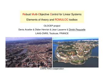
Robust Multi-Objective Control for Linear Systems Elements of theory and RoMulOC toolbox Denis Arzelier & Dimitri Peaucelle LAAS-CNRS, Toulouse, FRANCE also with Guilherme Chevarria, Alberto Bortott, Maud Sevin Introduction Robust
Robust Multi-Objective Control for Linear Systems Elements of theory and RoMulOC toolbox Denis Arzelier & Dimitri Peaucelle LAAS-CNRS, Toulouse, FRANCE also with Guilherme Chevarria, Alberto Bortott, Maud Sevin
Introduction ■ Robust control theory ● Robustness properties of the feedback loop ● Aim for guaranteed properties (stability and performances) ● Uncertain modeling of systems: tradeoff between complexity of systems & simplicity of models ■ Optimization based tools ● Linear Matrix Inequalities (LMI) framework [1990’s] ● Efficient fast solvers and nice parser for Matlab [2000’s] ● Possibility of a tool gathering established results : RoMulOC October 2009, Florian´ Seminar at UFSC 1 opolis
Outline ➊ Uncertain LTI systems and performances ● Control objectives: stability, transient response, perturbation rejection... ● Structured parametric uncertainties: extremal values, bounded sets... ➋ LMIs and convex polynomial-time optimization ● Semi-Definite Programming and LMIs ● SDP solvers and parsers ➌ Conservative LMI results ● Methods: Lyapunov, S-procedure, Finsler lemma, Topologic Separation... ● The ROMULOC toolbox October 2009, Florian´ Seminar at UFSC 2 opolis
➊ Uncertain LTI systems and performances ■ Linear Time-Invariant State-Space Multi-Input Multi-Output models ϑ [ x ]( t ) = Ax ( t ) + B u u ( t ) ϑ [ η ]( t ) = K A η ( t ) + K B y ( t ) , y ( t ) = C y x ( t ) + D yu u ( t ) u ( t ) = K C η ( t ) + K D y ( t ) x ∈ C n u ∈ C q u y ∈ C p y η ∈ C n K ● Continuous ( ϑ [ x ]( t ) = ˙ x ( t ) ) and discrete-time ( ϑ [ x ]( t ) = x ( t + T ) ) ■ analysis problem: For given ( K A , K B , K C , K D ) prove closed-loop properties of x x ( t ) = A ( K ) ( t ) ϑ η η ■ Design problem: Find ( K A , K B , K C , K D ) providing closed loop properties ● For n k = 0 : Static output-feedback (SOF) ● For n k = 0 and y = x : State feedback problem ● For n k = n : full order output-feedback problem October 2009, Florian´ Seminar at UFSC 3 opolis
➊ Uncertain LTI systems and performances ■ Control objectives ● Stability of ϑ [ x ]( t ) = A ( K ) x ( t ) ▲ For continuous-time: poles are all in left-hand half of complex plane ▲ For discrete-time: poles are all in unit circle of complex plane ● D R -Stability of ϑ [ x ]( t ) = A ( K ) x ( t ) : ▲ Poles are in region defined by D R = { s ∈ C : r 11 + sr 12 + s ∗ r 12 + ss ∗ r 22 ≤ 0 } , R = ( r ij ) Such regions are half-planes and discs 0 1 − 1 0 − 2 α cos ψ cos ψ − i sin ψ R = R = R = 1 0 0 1 cos ψ + i sin ψ 0 ψ α October 2009, Florian´ Seminar at UFSC 4 opolis
➊ Uncertain LTI systems and performances ■ Input/output objectives w ∈ C q w ϑ [ x ]( t ) = A ( K ) x ( t ) + B w ( K ) w ( t ) : z ∈ C p z z ( t ) = C z ( K ) x ( t ) + D zw ( K ) w ( t ) � ∞ ( � w � 2 = w ∗ wdt ) ● Induced L 2 gain: � z � ≤ γ ∞ � w � , 0 Also known as: H ∞ performance (max singular value H ( jω ) , ω ∈ R ), Robustness to unmodeled dynamics w = ∆ z , � ∆ � ≤ 1 /γ ∞ (bounded-real lemma) ● Impulse-to-norm performance: � z � ≤ γ 2 if w ( t ) = δ ( t ) 1 Also known as: H 2 performance (mean value H ( jω ) , ω ∈ R ), Energy of output in response to Gaussian white noise Norm-to-peak performance ( max | z | ≤ γ 2 � w � , z ∈ R ) ● Impulse-to-peak performance: max | z | ≤ γ i2p if w ( t ) = δ ( t ) α, � α � ≤ 1 . Also known as: Invariant ellipsoids Non saturating initial conditions October 2009, Florian´ Seminar at UFSC 5 opolis
➊ Uncertain LTI systems and performances ■ Robust Multi-Objective Control ● ∆ : errors in modeling, operating conditions, mass-production... ● ∆ : parametric uncertainty, assumed constant, belongs to a set ∆ ∆ . ϑ [ x ]( t ) = A (∆ , K ) x ( t ) + B w (∆ , K ) w ( t ) z ( t ) = C z (∆ , K ) x ( t ) + D zw (∆ , K ) w ( t ) ■ Design: Find a controller K that fulfills all robust specifications Π p =1 ... ¯ p defined for models Σ p (∆ p ) subject to uncertainties ∆ p ∈ ∆ ∆ p . F 2 (∆ ) F Σ (0) Σ 2 (∆ ) Σ 1 1 1 1 2 K K K ■ Analysis: For given K prove for each Σ p =1 ... ¯ p (∆ p ) that the specification Π p holds for all uncertainties ∆ p ∈ ∆ ∆ p . October 2009, Florian´ Seminar at UFSC 6 opolis
➊ Uncertain LTI systems and performances ■ Uncertain LTI systems: Affine with scalar parametric uncertainty [2] Σ Σ(∆) ● Polytopic models z w [1] Σ [v] Σ < γ u y K Convex hull of ¯ v vertices v =1 ξ v A [ v ] , B w (∆) = � ¯ A (∆) = � ¯ : ξ v ≥ 0 , � ¯ v =1 ξ v B [ v ] v v v . . . v =1 ξ v = 1 w ▲ Example: Linear combination of linear models identified on different operating points. ▲ The ξ v parameters may not have physical meaning ▲ ¯ v vertices can define a volume in ¯ v − 1 space of parameters (possible to divide space in polytopes with low number of vertices) October 2009, Florian´ Seminar at UFSC 7 opolis
➊ Uncertain LTI systems and performances ■ Uncertain LTI systems: Affine with scalar parametric uncertainty [2] Σ Σ(∆) ● Polytopic models z w [1] Σ [v] Σ < γ u y K Convex hull of ¯ v vertices A (∆) = � ¯ v =1 ξ v A [ v ] , : ξ v ≥ 0 , � ¯ v v . . . v =1 ξ v = 1 [0] Σ ● Parallelotopic models with ¯ ς axes z w Σ(∆) < γ u y K A (∆) = A | 0 | + � ¯ ς =1 δ ς A | ς | , ς . . . : | δ ς | ≤ 1 ▲ ¯ ς independent parameters δ ς identified in intervals ς vertices v = 2 ¯ ▲ polytope with ¯ October 2009, Florian´ Seminar at UFSC 8 opolis
➊ Uncertain LTI systems and performances ■ Uncertain LTI systems: Affine with scalar parametric uncertainty [0] Σ ● Parallelotopic models with ¯ ς axes z w Σ(∆) < γ u y K A (∆) = A | 0 | + � ¯ ς =1 ξ ς A | ς | , ς . . . : | ξ ς | ≤ 1 Σ(∆) ● Interval models with ¯ ς non-equal coefficients z w < γ u y K A � A (∆) � A : a ij ≤ a ij (∆) ≤ a ij . . . ▲ Parallelotope with axes in the euclidian basis of matrices ▲ All coefficients independent ▲ Change of basis does not preserve the structure October 2009, Florian´ Seminar at UFSC 9 opolis
➊ Uncertain LTI systems and performances ● Polytopic models can also be written as C [1] ξ 1 1 q 1 0 ∆ � � . ... B [1] B [¯ v ] A (∆) = A + . . . . . ∆ ∆ � �� � C [¯ v ] ξ ¯ 0 v 1 q ¯ B ∆ ∆ v � �� � � �� � ∆ C ∆ where for each vertex A [ v ] = A + B [ v ] ∆ C [ v ] ∆ with B [ v ] ∆ ∈ C n × q v . ● Parallelotopic models can also be written as C | 1 | δ 1 1 p 1 0 ∆ � � . ... A (∆) = A | 0 | B | 1 | B | ¯ ς | + . . . . . ∆ ∆ ���� � �� � A C | ¯ ς | δ ¯ 0 ς 1 p ¯ B ∆ ∆ ς � �� � � �� � ∆ C ∆ where for each axis A | ς | = B | ς | ∆ C | ς | ∆ with B | ς | ∆ ∈ C n × p ς . ▲ Factorisation as A (∆) = A + B ∆ ∆ C ∆ is not unique. October 2009, Florian´ Seminar at UFSC 10 opolis
➊ Uncertain LTI systems and performances ■ Uncertain LTI systems: Linear Fractional Representation (LFR) ∆ w z ∆ ∆ w z Σ < γ u y K ϑ [ x ]( t ) = Ax ( t ) + B ∆ w ∆ ( t ) + B w w ( t ) + B u u ( t ) w ∆ ∈ C q ∆ z ∆ ( t ) = C ∆ x ( t ) + D ∆∆ w ∆ ( t ) + D ∆ w w ( t ) + D ∆ u u ( t ) : z ∆ ∈ C p ∆ z ( t ) = C z x ( t ) + D z ∆ w ∆ ( t ) + D zw w ( t ) + D zu u ( t ) y ( t ) = C y x ( t ) + D y ∆ w ∆ ( t ) + D yw w ( t ) + D yu u ( t ) Linear - Fractional Transformation (LFT): A (∆) = A + B ∆ ∆( 1 − D ∆∆ ∆) − 1 C ∆ = A + B ∆ ( 1 − ∆ D ∆∆ ) − 1 ∆ C ∆ , B w (∆) = B w + B ∆ ∆( 1 − D ∆∆ ∆) − 1 D ∆ w . . . October 2009, Florian´ Seminar at UFSC 11 opolis
➊ Uncertain LTI systems and performances ■ Uncertain LTI systems: Linear Fractional Representation (LFR) ∆ w z ∆ ∆ w z Σ < γ u y K A (∆) = A + B ∆ ∆( 1 − D ∆∆ ∆) − 1 C ∆ = A + B ∆ ( 1 − ∆ D ∆∆ ) − 1 ∆ C ∆ . . . ● For any model where A (∆) , . . . are rational functions of δ j the LFT exists ● ∆ can always be taken as a bloc-diagonal matrix with repeated blocs 1 r 1 ⊗ ∆ 1 0 ... ∆ = 0 1 r ¯ j ⊗ ∆ ¯ j ▲ For scalar uncertainties 1 r j ⊗ δ j = δ j 1 r j ▲ LFR are not unique October 2009, Florian´ Seminar at UFSC 12 opolis
➊ Uncertain LTI systems and performances ■ Sets of uncertainties in LFRs ● { X, Y, Z }− dissipative uncertain matices � j Y ∗ + ∆ ∗ � : X + Y ∆ j + ∆ ∗ ∆ j j Z ∆ j ≤ 0 , X ≤ 0 , Z ≥ 0 ▲ Norm-bounded : � ∆ j � ≤ ρ 1 (gain limited operators) ➾ {− ρ 2 1 , 0 , 1 }− dissipative ▲ Positive real : ∆ j + ∆ ∗ j ≥ 0 (passive operators) ➾ { 0 , − 1 , 0 }− dissipative October 2009, Florian´ Seminar at UFSC 13 opolis
Recommend
More recommend
Explore More Topics
Stay informed with curated content and fresh updates.
