Robust Multi-Objective Control for Linear Systems Elements of theory - - PowerPoint PPT Presentation

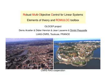
Robust Multi-Objective Control for Linear Systems Elements of theory and ROMULOC toolbox

Dimitri PEAUCELLE & Denis ARZELIER LAAS-CNRS, Toulouse, FRANCE with the participation of Master’s Students Maud SEVIN & Alberto BORTOTT

General Features of RoMulOC ➞ Matlab Toolbox - freely distributed www/laas.fr/OLOCEP/romuloc

I - Modeling features of uncertain LTI systems

➞ State-space systems with performance input/output channel ➞ Both polytopic and LFT uncertain systems - large variety of uncertainty models ➞ Basic model manipulations

II - Robust performances in Lyapunov framework

➞ Robust control objectives: stability, transient response (pole location),

perturbation rejection (H∞, H2 and impulse-to-peak)

➞ All performances are recast in a Lyapunov framework ➞ Robustness is achieved with either Unique Lyapunov function or PDLF ➞ LMI results derived using Quadratic Separation and Slack Variables

III - LMIs and convex polynomial-time optimization

➞ Semi-Definite Programming and LMIs (black box) ➞ SDP solvers and YALMIP parser (user can tune solvers)

RoMulOC toolbox 1 WCFCL ’08, September 26th, 2008, Sienna

Demo example - problem formulation

6-th order mechanical system (x ∈ R3)

¨ x(t) + M −1(∆M)D(∆D) ˙ x(t) + M −1(∆M)Kx(t) = M −1(∆M)E(∆E)w(t) z(t) = C(∆C)x(t) + Fw(t)

where

M(∆M) = M0 + M1∆MM2 with ∆M ∈ R1×2 in ellipsoid

0.35 0.3 0.25 0.2 0.15 0.1 0.05 0.05 0.1 0.15 0.15 0.1 0.05 0.05 0.1 0.15 0.2 0.25 0.3 0.35

D(∆D) = D0 + D1∆DD2 with ∆D ∈ R2×2 norm-bounded ∆T

D∆D ≤ 0.252I

E(∆E) = E0 + E1∆EE2 with ∆E ∈ [−0.25 0.25] scalar in interval C(∆C) = C0 + C1∆CC2 with ∆C ∈ R2×2 in polytope co

• ∆[1]

C , ∆[2] C , ∆[3] C

• Robust analysis

➞ Robust pole location in a sector (robust bound on damping of all modes) ➞ Robust H∞ norm of w → z transfer : Tz/w(s, ∆)∞ ≤ γ.

RoMulOC toolbox 2 WCFCL ’08, September 26th, 2008, Sienna

Demo example - solved with RoMulOC

>> sys=ssmodel(’mechanical system’); >> sys.A = [ zeros(n) , eye(n) ; -iM0*D0 , -iM0*K ]; ... >> sys.Bw = [ zeros(n) ; iM0*E0 ]; >> Dm = udiss( X, Y, Z, ’Inertia’); >> Dd = unb( 2, 2, 0.25, ’Damping’); >> De = uinter(-0.25, 0.25, ’Input’); >> Dc = upoly( Dcv, ’Output’); >> usys = ussmodel( sys, diag(Dm, Dd, De, Dc) ); >> r1 = region( ’plane’, 0, asin(0.35) ); >> pb1 = dstability( usys, r1 ); >> pb1 = pb1 + ctrpb( ’analysis’, ’Lyap unique’ ); >> IsDstable = solvesdp( pb1 ); >> pb2 = hinfty( pb2, usinf ); >> pb2unique = pb2 + ctrpb( ’analysis’, ’Lyap unique’ ); >> HinfLyapUnique = solvesdp( pb2unique ); >> pb2PDLF = pb2 + ctrpb( ’analysis’ , ’PDLF’ ); >> HinfPDLF = solvesdp( pb2PDLF );

RoMulOC toolbox 3 WCFCL ’08, September 26th, 2008, Sienna

I - Uncertain LTI systems and performances

General Robust Multi-Objective Control Problem

∆ : errors in modeling, operating conditions, mass-production... ∆ : uncertainty belongs to a set ∆ ∆. sx(t) = A(∆)x(t) + Bw(∆)w(t) + Bu(∆)u(t) z(t) = Cz(∆)x(t) + Dzw(∆)w(t) + Dzu(∆)u(t) y(t) = Cy(∆)x(t) + Dyw(∆)w(t) + Dyu(∆)u(t)

Find controller K that fulfills robust specifications Πi defined for models Σi(∆i) with ∆i ∈ ∆

∆i.

K Σ2 F2 (Δ )

2

K

1

(Δ )

1

K

1

Σ (0)

1

F Σ

RoMulOC today

➞ Modeling tools ready for the global design problem (uncertainties restricted to be constant) ➞ Analysis : Unique Lyapunov function and a PDLF method ➞ Control design : only for unique Lyapunov function

RoMulOC toolbox 4 WCFCL ’08, September 26th, 2008, Sienna

I - Uncertain LTI systems and performances ➞ Polytopic models

z w K u y < γ

[2]

Σ Σ

[1]

Σ

[N]

Σ(Δ)

✪ Affine polytopic models : convex hull of N vertices A(∆) = ζiA[i] , Bw(∆) = ζiB[i]

w

. . . : ζi ≥ 0 , ζi = 1

RoMulOC toolbox 5 WCFCL ’08, September 26th, 2008, Sienna

I - Uncertain LTI systems and performances ➞ Polytopic models

z w K u y < γ

[2]

Σ Σ

[1]

Σ

[N]

Σ(Δ)

✪ Affine polytopic models : convex hull of N vertices A(∆) = ζiA[i] , Bw(∆) = ζiB[i]

w

. . . : ζi ≥ 0 , ζi = 1 ➥ Parallelotopic models with NP axes A(∆) = A[0] + ξiA[i] , Bw(∆) = B[0]

w + ξiB[i] w

. . . : |ξi| ≤ 1 ➾ polytope with N = 2NP vertices ➥ Interval models with NI non equal coefficients A[1] A(∆) A[2] : a[1]

ij ≤ aij(∆) ≤ a[2] ij

➾ parallelotope with axes in the euclidian basis of matrices ➾ polytope with N = 2NI vertices

RoMulOC toolbox 6 WCFCL ’08, September 26th, 2008, Sienna

I - Uncertain LTI systems and performances ➞ LFT models

z

Σ Δ

w z K y u < γ w

Δ Δ

sx(t) = Ax(t) + B∆w∆(t) + Bww(t) + Buu(t) z∆(t) = C∆x(t) + D∆∆w∆(t) + D∆ww(t) + D∆uu(t) z(t) = Czx(t) + Dz∆w∆(t) + Dzww(t) + Dzuu(t) y(t) = Cyx(t) + Dy∆w∆(t) + Dyww(t) + Dyuu(t) : w∆ ∈ Cq∆ z∆ ∈ Cp∆

Linear - Fractional Transformation:

A(∆) = A+B∆∆(I−D∆∆∆)−1C∆ , Bw(∆) = Bw+B∆∆(I−D∆∆∆)−1D∆w . . .

Any model rational in δi parameters ➾ LFT (not unique) with diagonal ∆ =diag(δ1, δ1, ..., δ2, ...). RoMulOC toolbox 7 WCFCL ’08, September 26th, 2008, Sienna

I - Uncertain LTI systems and performances ➞ Uncertainty sets ✪ {X, Y, Z}−dissipative matrices

• ∆ ∈ Cqw×pz

: X + Y ∆ + ∆∗Y ∗ + ∆∗Z∆ ≤ O , X ≤ O , Z ≥ O

• ➥ Norm-bounded uncertainties : ∆ ≤ ρ1

➾ {−ρ2I, O, I}−dissipative ➥ Positive real uncertainties : ∆ + ∆∗ ≥ O (eg. s) ➾ {O, −I, O}−dissipative

RoMulOC toolbox 8 WCFCL ’08, September 26th, 2008, Sienna

I - Uncertain LTI systems and performances ➞ Uncertainty sets ✪ {X, Y, Z}−dissipative matrices

• ∆ ∈ Cqw×pz

: X + Y ∆ + ∆∗Y ∗ + ∆∗Z∆ ≤ O , X ≤ O , Z ≥ O

• ➥ Norm-bounded uncertainties : ∆ ≤ ρ1

➾ {−ρ2I, O, I}−dissipative ➥ Positive real uncertainties : ∆ + ∆∗ ≥ O (eg. s) ➾ {O, −I, O}−dissipative ✪ Polytopic uncertainties

polytope N vertices

• ∆ = ζi∆[i] : ζi ≥ 0 , ζi = 1
• ➥ Parallelotopic uncertainties

NP axes ➾

polytope N = 2NP

• ∆ = ∆[0] + ξi∆[i] : |ξi| ≤ 1
• ➥ Interval uncertainties

NI coef. = ➾

polytope N = 2NI

• ∆[1] ∆ ∆[2] : δ[1]

ij ≤ δij ≤ δ[2] ij

• RoMulOC toolbox

9 WCFCL ’08, September 26th, 2008, Sienna

Demo example - solved with RoMulOC

>> sys=ssmodel(’mechanical system’); >> sys.A = [ zeros(n) , eye(n) ; -iM0*D0 , -iM0*K ]; ... >> sys.Bw = [ zeros(n) ; iM0*E0 ]; >> Dm = udiss( X, Y, Z, ’Inertia’); >> Dd = unb( 2, 2, 0.25, ’Damping’); >> De = uinter(-0.25, 0.25, ’Input’); >> Dc = upoly( Dcv, ’Output’); >> usys = ussmodel( sys, diag(Dm, Dd, De, Dc) ); >> r1 = region( ’plane’, 0, asin(0.35) ); >> pb1 = dstability( usys, r1 ); >> pb1 = pb1 + ctrpb( ’analysis’, ’Lyap unique’ ); >> IsDstable = solvesdp( pb1 ); >> pb2 = hinfty( pb2, usinf ); >> pb2unique = pb2 + ctrpb( ’analysis’, ’Lyap unique’ ); >> HinfLyapUnique = solvesdp( pb2unique ); >> pb2PDLF = pb2 + ctrpb( ’analysis’ , ’PDLF’ ); >> HinfPDLF = solvesdp( pb2PDLF );

RoMulOC toolbox 10 WCFCL ’08, September 26th, 2008, Sienna

II - Lyapunov based analysis

Nominal performance analysis V (x) = xT Px Lyapunov function (P > O)

✪ Stability AT P + PA < O | AT PA − P < O ✪ D-Stability

• I

A∗

• 

 r11P r12P r∗

12P

r22P     I A   < O ✪ H∞ norm   AT P + PA + CT

z Cz

PBw + CT

z Dzw

BT

wP + DT zwCz

−γ2I + DT

zwDzw

  < O ✪ H2 norm AT P + PA + CT

z Cz < O

trace(BT

wPBw) < γ2

✪ Impulsion-to-peak AT P + PA < O BT

wPBw < γ2I

CT

z Cz < P

DT

zwDzw < γ2I

RoMulOC toolbox 11 WCFCL ’08, September 26th, 2008, Sienna

II - Lyapunov based analysis

Robust performance analysis V (x, ∆) parameter-dependent Lyapunov function.

✪ Nominal analysis (LMI) → Robust analysis (NP-hard) ∃ P : LΣ(P) < O → ∀ ∆ ∈ ∆ ∆ , ∃ P(∆) : LΣ(∆)(P(∆)) < O

Test over sample values in ∆

∆ gives optimistic results.

RoMulOC toolbox 12 WCFCL ’08, September 26th, 2008, Sienna

II - Lyapunov based analysis

Robust performance analysis V (x, ∆) parameter-dependent Lyapunov function.

✪ Nominal analysis (LMI) → Robust analysis (NP-hard) ∃ P : LΣ(P) < O → ∀ ∆ ∈ ∆ ∆ , ∃ P(∆) : LΣ(∆)(P(∆)) < O

Test over sample values in ∆

∆ gives optimistic results. ➥ Choice of P(∆) for having a finite number of decision variables

(and, conservative, techniques to have finite nb of LMIs)

➙ “Quadratic Stability”: P(∆) = P ➙ Polytopic PDLF: P(∆) = ζiP [i]

(and ”Slack Variables” technique)

➙ Quadratic-LFT PDLF:

(and Quadratic Separation)

P(∆) =

• I

∆T

C

• P

  I ∆C   , ∆C = (I − ∆D∆∆)−1∆C∆

RoMulOC toolbox 13 WCFCL ’08, September 26th, 2008, Sienna

Demo example - solved with RoMulOC

>> sys=ssmodel(’mechanical system’); >> sys.A = [ zeros(n) , eye(n) ; -iM0*D0 , -iM0*K ]; ... >> sys.Bw = [ zeros(n) ; iM0*E0 ]; >> Dm = udiss( X, Y, Z, ’Inertia’); >> Dd = unb( 2, 2, 0.25, ’Damping’); >> De = uinter(-0.25, 0.25, ’Input’); >> Dc = upoly( Dcv, ’Output’); >> usys = ussmodel( sys, diag(Dm, Dd, De, Dc) ); >> r1 = region( ’plane’, 0, asin(0.35) ); >> pb1 = dstability( usys, r1 ); >> pb1 = pb1 + ctrpb( ’analysis’, ’Lyap unique’ ); >> IsDstable = solvesdp( pb1 ); >> pb2 = hinfty( pb2, usinf ); >> pb2unique = pb2 + ctrpb( ’analysis’, ’Lyap unique’ ); >> HinfLyapUnique = solvesdp( pb2unique ); >> pb2PDLF = pb2 + ctrpb( ’analysis’ , ’PDLF’ ); >> HinfPDLF = solvesdp( pb2PDLF );

RoMulOC toolbox 14 WCFCL ’08, September 26th, 2008, Sienna

III - LMIs and convex polynomial-time optimization

Semi-Definite Programming and LMIs

➞ The LMI problem is defined in YALMIP format ➞ Can be solved with any available SDP software result = solvesdp( problem , sdpsettings(’solver’, ’sdpt3’)) ➞ result is the answer to the problem, e.g. the guaranteed H∞ norm ➞ Constraints and variables are also available problem.vars problem.lmi

Results for the demo example with SeDuMi solver Nominal 200 rand. val. 2000 rand. val. Robust PDLF Unique Lyapunov

H∞

2 2.484 2.4957 ?? 2.516 2.866 time

0.036s 13.79s

2 min NP

17.99s 6.772s

RoMulOC toolbox 15 WCFCL ’08, September 26th, 2008, Sienna

Conclusions and Prospective work

Tests and users feedback

➞ Test yourself : www.laas.fr/OLOCEP/romuloc/ ➞ Tests done at LAAS with fitted to application improvements

(clearance of satellite attitude & flight control laws) Future versions

➞ PDLF State-feedback design

• soon some first results

➞ Output-feedback : full-order (LMI) and SOF (BMI)

• not planned

➞ Uncertain Time-Delay Systems (F

. Gouaisbaut)

• possible

➞ Discrete-time uncertain Periodic Systems (C. Farges)

• not planned

➞ Time varying uncertainties

• work in progress

➞ Uncertain Descriptor Systems

• work in progress

RoMulOC toolbox 16 WCFCL ’08, September 26th, 2008, Sienna

Conclusions and Prospective work

Uncertain descriptor systems: a method for more PDLF, less conservative, results

➞ PDLF stability analysis of ˙ x = A(∆)x with V (x, ∆) = xT P(∆)x where P(∆) =

• I

AT (∆)

• P

  I A(∆)   ➞ is equivalent to ”Lyapunov unique” stability analysis with V (x, ˙ x) =

• x

˙ x

• P

  x ˙ x  

• f the augmented system, in descriptor form:

    I O O I I O       ˙ x ¨ x   =     A(∆) O O A(∆) O I       x ˙ x   ➚ Reducing conservatism is as simple as augmenting the model with higher order derivatives ➘ Needs to produce and code LMI results for descriptor systems (work in progress)

RoMulOC toolbox 17 WCFCL ’08, September 26th, 2008, Sienna

Conclusions and Prospective work

Uncertain descriptor systems: extensions for time-vaying uncertainties, delays ...

➞ For a time-varying uncertainty, model augmentation by derivation produces: w∆ = ∆z∆ ˙ w∆ = ˙ ∆z∆ + ∆ ˙ z∆ ➞ For delays, similar procedure produces new Lyapunov-Krasovskii results: e−sh = 1 − sh + (sh)2

2

+ . . . ↓ x(t − h) = x(t) − h ˙ x(t) + h2

2 ¨

x(t) + . . . ➞ Possible extensions for the case when ∆ is a non-linear operator ?

RoMulOC toolbox 18 WCFCL ’08, September 26th, 2008, Sienna