Regression with Many Predictors 21.12.2016 Goals of Todays Lecture - PowerPoint PPT Presentation
Regression with Many Predictors 21.12.2016 Goals of Todays Lecture Get a (limited) overview of different approaches to handle data-sets with (many) more variables than observations. 1 / 9 Linear model in high dimensions Example Can the
Regression with Many Predictors 21.12.2016
Goals of Today’s Lecture Get a (limited) overview of different approaches to handle data-sets with (many) more variables than observations. 1 / 9
Linear model in high dimensions Example Can the concentration of a (specific) component be predicted from spectra? Can the yield of a plant be predicted from its gene expression data? We have ◮ a response variable Y (yield) ◮ many predictor variables x (1) , . . . , x ( m ) (gene expr.) The easiest model is a linear model. Y i = x i β 0 + E i i = 1 . . . n , But... we typically have many more predictor variables than observations ( m > n )! I.e. the model is high-dimensional 2 / 9
Linear model in high dimensions High-dimensional models are more problematic because we can not compute the linear regression. If we want to use all predictor variables, we can’t fit the model because it would give a perfect fit. Mathematically, the matrix ( X T X ) ∈ R m × m can not be inverted. � Therefore, we need methods that can deal with this new situation. 3 / 9
Stepwise Forward Selection of Variables A simple approach is stepwise forward regression . It works as follows: Start with empty model, only consisting of intercept. Add the predictor to the model that has the smallest p-value . For that reason fit all models with just one predictor and compare p-values. Add all possible predictors to the model of the last step, expand the model with the one with smallest p-value. Continue until some stopping criterion is met. Pro’s: Easy Con’s: Unstable: small perturbation of data can lead to (very) different results, may miss“best”model. 4 / 9
Principal Component Regression Idea: Perform PCA on (centered) design matrix X . PCA will give us a“new”design matrix Z . Use first p < m columns. Perform an ordinary linear regression with the“new data” . Pro’s New design matrix Z is orthogonal (by construction). Con’s We have not used Y when doing PCA. It could very well be that some of the“last”principal components are useful for predicting Y ! Extension Select those principal components that have largest (simple) correlation with the response Y . 5 / 9
Ridge Regression Ridge regression“shrinks”the regression coefficients by adding a penalty to the least squares criterion. m � � � Y − X β � 2 β 2 β λ = arg min 2 + λ , j β j =1 where λ ≥ 0 is a tuning parameter that controls the size of the penalty. The first term is the usual residual sum of squares. The second term penalizes the coefficients. Intuition: Trade-off between goodness of fit (first-term) and penalty (second term). 6 / 9
Ridge Regression There is a closed form solution � β λ = ( X T X + λ I ) − 1 X T Y , where I is the identity matrix. Even if X T X is singular, we have a unique solution because we add the diagonal matrix λ I . λ is the tuning parameter ◮ For λ = 0 we have the usual least squares fit (if it exists). ◮ For λ → ∞ we have � β λ → 0 (all coefficients shrunken to zero in the limit). 7 / 9
Lasso Lasso = L east A bsolute S hrinkage and S election O perator. This is similar to Ridge regression, but“more modern” . m � � � Y − X β � 2 β λ = arg min 2 + λ | β j | , β j =1 It has the property that it also selects variables, i.e. many components of � β λ are zero (for large enough λ ). 8 / 9
Statistical Consulting Service Get help/support for planning your experiments. doing proper analysis of your data to answer your scientific questions. Information available at http://stat.ethz.ch/consulting 9 / 9
Recommend
More recommend
Explore More Topics
Stay informed with curated content and fresh updates.



![CS480/680 Machine Learning Lecture 3: May 13, 2019 Linear Regression [RN] Sec. 18.6.1, [HTF]](https://c.sambuz.com/988148/cs480-680-machine-learning-lecture-3-may-13-2019-s.webp)
