Comparing Nested Models Two regression models are called nested if - PowerPoint PPT Presentation

ST 370 Probability and Statistics for Engineers Comparing Nested Models Two regression models are called nested if one contains all the predictors of the other, and some additional predictors. For example, the first-order model in two independent variables, Y = β 0 + β 1 x 1 + β 2 x 2 + ǫ, is nested within the complete second-order model Y = β 0 + β 1 x 1 + β 2 x 2 + β 11 x 2 1 + β 22 x 2 2 + β 12 x 1 x 2 + ǫ. How to choose between them? 1 / 17 Multiple Linear Regression

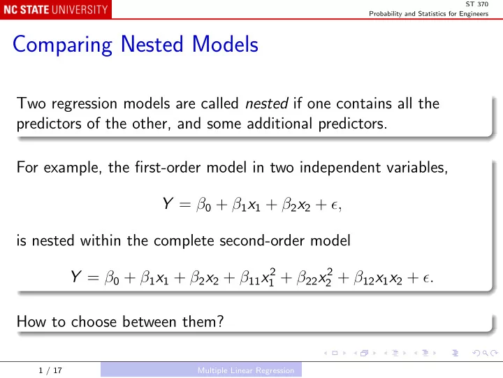
ST 370 Probability and Statistics for Engineers If the models are being considered for making predictions about the mean response or about future observations, you could just use PRESS or P 2 . But you may be interested in whether the simpler model is adequate as a description of the relationship, and not necessarily in whether it gives better predictions. 2 / 17 Multiple Linear Regression

ST 370 Probability and Statistics for Engineers A single added predictor If the larger model has just one more predictor than the smaller model, you could just test the significance of the one additional coefficient, using the t -statistic. Multiple added predictors When the models differ by r > 1 added predictors, you cannot compare them using t -statistics. The conventional test is based on comparing the regression sums of squares for the two models: the general regression test , or the extra sum of squares test. 3 / 17 Multiple Linear Regression

ST 370 Probability and Statistics for Engineers Write SS R , reduced and SS R , full for the regression sums of squares of the two models, where the “reduced” model is nested within the “full” model. The extra sum of squares is SS R , extra = SS R , full − SS R , reduced and if this is large, the r additional predictors have explained a substantial additional amount of variability. We test the null hypothesis that the added predictors all have zero coefficients using the F -statistic F obs = SS R , extra / r . MS E , full 4 / 17 Multiple Linear Regression

ST 370 Probability and Statistics for Engineers In R The R function anova() (not to be confused with aov() ) implements the extra sum of squares test: wireBondLm2 <- lm(Strength ~ Length + I(Length^2) + Height, wireBond) wireBondLm3 <- lm(Strength ~ Length + I(Length^2) + Height + I(Height^2) + I(Length * Height), wireBond) anova(wireBondLm1, wireBondLm3) It can also compare a sequence of more than two nested models: anova(wireBondLm1, wireBondLm2, wireBondLm3) 5 / 17 Multiple Linear Regression

ST 370 Probability and Statistics for Engineers Note Because SS R = SS T − SS E and SS T is the same for all models, the extra sum of squares can also be written SS R , extra = SS E , reduced − SS E , full That is, the extra sum of squares is also the amount by which the residual sum of squares is reduced by the additional predictors. Note The nested model F -test can also be used when r = 1, and is equvalent to the | t | -test for the added coefficient, because F = t 2 . 6 / 17 Multiple Linear Regression

ST 370 Probability and Statistics for Engineers Indicator Variables Recall that an indicator variable is a variable that takes only the values 0 and 1. A single indicator variable divides the data into two groups, and is a quantitative representation of a categorical factor with two levels. To represent a factor with a > 2 levels, you need a − 1 indicator variables. 7 / 17 Multiple Linear Regression

ST 370 Probability and Statistics for Engineers Recall the paper strength example: the factor is Hardwood Concentration, with levels 5%, 10%, 15%, and 20%. Define indicator variables � 1 for 5% hardwood x 1 = 0 otherwise � 1 for 10% hardwood x 2 = 0 otherwise � 1 for 15% hardwood x 3 = 0 otherwise � 1 for 20% hardwood x 4 = 0 otherwise 8 / 17 Multiple Linear Regression

ST 370 Probability and Statistics for Engineers Consider the regression model Y i = β 0 + β 2 x i , 2 + β 3 x i , 3 + β 4 x i , 4 + ǫ i . The interpretation of β 0 is, as always, the mean response when x 2 = x 3 = x 4 = 0; in this case, that is for the remaining (baseline) category, 5% hardwood. For 10% hardwood, x 2 = 1 and x 3 = x 4 = 0, so the mean response is β 0 + β 2 ; the interpretation of β 2 is the difference between the mean responses for 10% hardwood and the baseline category. 9 / 17 Multiple Linear Regression

ST 370 Probability and Statistics for Engineers Similarly β 3 is the difference between 15% hardwood and the baseline category, and β 4 is the difference between 20% hardwood and the baseline category. So the interpretations of β 0 , β 2 , β 3 , and β 4 are exactly the same as the interpretations of µ , τ 2 , τ 3 , and τ 4 in the one-factor model Y i , j = µ + τ i + ǫ i , j . The factorial model may be viewed as a special form of regression model with these indicator variables as constructed predictors. Modern statistical software fits factorial models using regression with indicator functions. 10 / 17 Multiple Linear Regression

ST 370 Probability and Statistics for Engineers Combining Categorical and Quantitative Predictors Example: surface finish The response Y is a measure of the roughness of the surface of a metal part finished on a lathe. Factors RPM; Type of cutting tool (2 types, 302 and 416). 11 / 17 Multiple Linear Regression

ST 370 Probability and Statistics for Engineers Begin with the model Y = β 0 + β 1 x 1 + β 2 x 2 + ǫ where x 1 is RPM and x 2 is the indicator for type 416: parts <- read.csv("Data/Table-12-11.csv") pairs(parts) parts$Type <- as.factor(parts$Type) summary(lm(Finish ~ RPM + Type, parts)) 12 / 17 Multiple Linear Regression

ST 370 Probability and Statistics for Engineers Call: lm(formula = Finish ~ RPM + Type, data = finish) Residuals: Min 1Q Median 3Q Max -0.9546 -0.5039 -0.1804 0.4893 1.5188 Coefficients: Estimate Std. Error t value Pr(>|t|) (Intercept) 14.276196 2.091214 6.827 2.94e-06 *** RPM 0.141150 0.008833 15.979 1.13e-11 *** Type416 -13.280195 0.302879 -43.847 < 2e-16 *** --- Signif. codes: 0 *** 0.001 ** 0.01 * 0.05 . 0.1 1 Residual standard error: 0.6771 on 17 degrees of freedom Multiple R-squared: 0.9924,Adjusted R-squared: 0.9915 F-statistic: 1104 on 2 and 17 DF, p-value: < 2.2e-16 13 / 17 Multiple Linear Regression

ST 370 Probability and Statistics for Engineers For tool type 302, x 2 = 0, so the fitted equation is y = 14 . 276 + 0 . 141 × RPM ˆ while for tool type 416, x 2 = 1, and the fitted equation is y = 14 . 276 − 13 . 280 + 0 . 141 × RPM ˆ = 0 . 996 + 0 . 141 × RPM We are essentially fitting parallel straight lines against RPM for the two tool types: the same slope, but different intercepts. 14 / 17 Multiple Linear Regression

ST 370 Probability and Statistics for Engineers We could also allow the slopes to be different: Y = β 0 + β 1 x 1 + β 2 x 2 + β 1 , 2 x 1 x 2 + ǫ. In this model, the slopes versus RPM are β 1 for type 302 and β 1 + β 1 , 2 for type 416. summary(lm(Finish ~ RPM * Type, parts)) 15 / 17 Multiple Linear Regression

ST 370 Probability and Statistics for Engineers Call: lm(formula = Finish ~ RPM * Type, data = finish) Residuals: Min 1Q Median 3Q Max -0.68655 -0.44881 -0.07609 0.30171 1.76690 Coefficients: Estimate Std. Error t value Pr(>|t|) (Intercept) 11.50294 2.50430 4.593 0.0003 *** RPM 0.15293 0.01060 14.428 1.37e-10 *** Type416 -6.09423 4.02457 -1.514 0.1495 RPM:Type416 -0.03057 0.01708 -1.790 0.0924 . --- Signif. codes: 0 *** 0.001 ** 0.01 * 0.05 . 0.1 1 Residual standard error: 0.6371 on 16 degrees of freedom Multiple R-squared: 0.9936,Adjusted R-squared: 0.9924 F-statistic: 832.3 on 3 and 16 DF, p-value: < 2.2e-16 16 / 17 Multiple Linear Regression

ST 370 Probability and Statistics for Engineers We do not reject the null hypothesis that the interaction term has a zero coefficient, so the fitted lines are not significantly different from parallel. 17 / 17 Multiple Linear Regression