Comparing Nested Models Two models are nested if one model contains - PowerPoint PPT Presentation

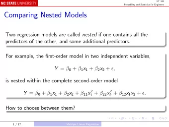
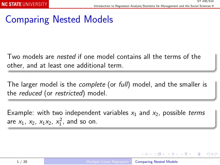
ST 430/514 Introduction to Regression Analysis/Statistics for Management and the Social Sciences II Comparing Nested Models Two models are nested if one model contains all the terms of the other, and at least one additional term. The larger model is the complete (or full ) model, and the smaller is the reduced (or restricted ) model. Example: with two independent variables x 1 and x 2 , possible terms are x 1 , x 2 , x 1 x 2 , x 2 1 , and so on. 1 / 20 Multiple Linear Regression Comparing Nested Models

ST 430/514 Introduction to Regression Analysis/Statistics for Management and the Social Sciences II Consider three models: First order: E ( Y ) = β 0 + β 1 x 1 + β 2 x 2 ; Interaction: E ( Y ) = β 0 + β 1 x 1 + β 2 x 2 + β 3 x 1 x 2 ; Full second order: E ( Y ) = β 0 + β 1 x 1 + β 2 x 2 + β 3 x 1 x 2 + β 4 x 2 1 + β 5 x 2 2 . 2 / 20 Multiple Linear Regression Comparing Nested Models

ST 430/514 Introduction to Regression Analysis/Statistics for Management and the Social Sciences II The first order model is nested within both the Interaction model and the Full second order model. The Interaction model is nested within the Full second order model. We usually want to use the simplest (most parsimonious ) model that adequately fits the observed data. One way to decide between a full model and a reduced model is by testing H 0 : reduced model is adequate; H a : full model is better. 3 / 20 Multiple Linear Regression Comparing Nested Models

ST 430/514 Introduction to Regression Analysis/Statistics for Management and the Social Sciences II When the full model has exactly one more term than the reduced model, we can use a t -test. E.g., testing the Interaction model E ( Y ) = β 0 + β 1 x 1 + β 2 x 2 + β 3 x 1 x 2 ; against the First order model E ( Y ) = β 0 + β 1 x 1 + β 2 x 2 . H 0 : “reduced model is adequate” is the same as H 0 : β 3 = 0. So the usual t -statistic is the relevant test statistic. 4 / 20 Multiple Linear Regression Comparing Nested Models

ST 430/514 Introduction to Regression Analysis/Statistics for Management and the Social Sciences II When the full model has more than one additional term, we use an F -test, which generalizes the t -test. Basic idea: fit both models, and test whether the full model fits significantly better than the reduced model: Drop in SSE � � Number of extra terms F = s 2 for full model where SSE is the sum of squared residuals. When H 0 is true, F follows the F -distribution, which we use to find the P -value. 5 / 20 Multiple Linear Regression Comparing Nested Models

ST 430/514 Introduction to Regression Analysis/Statistics for Management and the Social Sciences II E.g., testing the (full) second order model E ( Y ) = β 0 + β 1 x 1 + β 2 x 2 + β 3 x 1 x 2 + β 4 x 2 1 + β 5 x 2 2 ; against the (reduced) interaction model E ( Y ) = β 0 + β 1 x 1 + β 2 x 2 + β 3 x 1 x 2 . Here H 0 is β 4 = β 5 = 0, and H a is the opposite. In R, the lm() method is not convenient for carrying out this test; aov() is better. 6 / 20 Multiple Linear Regression Comparing Nested Models

ST 430/514 Introduction to Regression Analysis/Statistics for Management and the Social Sciences II summary(aov(Cost ~ Weight + Distance + I(Weight * Distance) + I(Weight^2) + I(Distance^2), express)) Df Sum Sq Mean Sq F value Pr(>F) Weight 1 270.55 270.55 1380.001 2.17e-15 *** Distance 1 143.63 143.63 732.616 1.72e-13 *** I(Weight * Distance) 1 31.27 31.27 159.487 4.84e-09 *** I(Weight^2) 1 3.80 3.80 19.383 0.000602 *** I(Distance^2) 1 0.09 0.09 0.451 0.512657 Residuals 14 2.74 0.20 --- Signif. codes: 0 *** 0.001 ** 0.01 * 0.05 . 0.1 1 summary(aov(Cost ~ Weight + Distance + I(Weight * Distance), express)) Df Sum Sq Mean Sq F value Pr(>F) Weight 1 270.55 270.55 652.59 2.14e-14 *** Distance 1 143.63 143.63 346.45 2.89e-12 *** I(Weight * Distance) 1 31.27 31.27 75.42 1.88e-07 *** Residuals 16 6.63 0.41 --- Signif. codes: 0 *** 0.001 ** 0.01 * 0.05 . 0.1 1 7 / 20 Multiple Linear Regression Comparing Nested Models

ST 430/514 Introduction to Regression Analysis/Statistics for Management and the Social Sciences II These are sequential sums of squares, adding each term to the model in order. See Residuals line in each set of results: SSE(Full second order) = 2 . 74 , SSE(Interaction) = 6 . 63 , so F = (6 . 63 − 2 . 74) / 2 = 9 . 75 , P < . 01 0 . 20 8 / 20 Multiple Linear Regression Comparing Nested Models

ST 430/514 Introduction to Regression Analysis/Statistics for Management and the Social Sciences II You can, in fact, calculate F from the output for the full model: Note that, because the terms are added sequentially, the sums of squares for the common terms ( Weight , Distance , and Weight * Distance ) are the same in both models. In the reduced model, the extra terms ( Weight^2 and Distance^2 ) have gone away. Their combined sum of squares, 3.80 + 0.09 = 3.89, is exactly the increase in SSE, 6.63 - 2.74 = 3.89. 9 / 20 Multiple Linear Regression Comparing Nested Models

ST 430/514 Introduction to Regression Analysis/Statistics for Management and the Social Sciences II So we can also calculate F = (Sum Sq for Weight^ 2 + Sum Sq for Distance^ 2 ) / 2 Mean Square for Residuals using only the output for the full model. Note that F was calculated imprecisely, because of rounding. We can get more digits using print(summary(...), digits = 8) for example, or calculate F to full precision: s <- summary(aov(Cost ~ Weight + Distance + I(Weight * Distance) + I(Weight^2) + I(Distance^2), express))[[1]] sum(s[c("I(Weight^2)", "I(Distance^2)"), "Sum Sq"]) / 2 / s["Residuals", "Mean Sq"] 10 / 20 Multiple Linear Regression Comparing Nested Models

ST 430/514 Introduction to Regression Analysis/Statistics for Management and the Social Sciences II We could use the same F -test when there is only one additional term in the full model, based on just one line in the ANOVA table, provided it is the last term in the formula. It appears very different from the t -test described earlier. Some matrix algebra shows that it is, in fact, exactly the same test: The F -statistic is exactly the square of the t -statistic. The F critical values are exactly the squares of the (two-sided) t critical values. So the P -value is exactly the same. 11 / 20 Multiple Linear Regression Comparing Nested Models

ST 430/514 Introduction to Regression Analysis/Statistics for Management and the Social Sciences II Complete Example: Road Construction Cost Data from the Florida Attorney General’s office y = successful bid; x 1 = DOT engineer’s estimate of cost x 2 = indicator of fixed bidding: � 1 if fixed x 2 = 0 if competitive 12 / 20 Multiple Linear Regression A Complete Example

ST 430/514 Introduction to Regression Analysis/Statistics for Management and the Social Sciences II Get the data and plot them: flag <- read.table("Text/Exercises&Examples/FLAG.txt", header = TRUE) pairs(flag[, -1]) Section 4.14 suggests beginning with the full second order model, and simplifying it as far as possible (but no further!). We’ll take the opposite approach: begin with the first order model, and complicate it as far as necessary. Because x 2 is an indicator variable, the first order model is a pair of parallel straight lines: summary(lm(COST ~ DOTEST + STATUS, flag)) 13 / 20 Multiple Linear Regression A Complete Example

ST 430/514 Introduction to Regression Analysis/Statistics for Management and the Social Sciences II First order model Call: lm(formula = COST ~ DOTEST + STATUS, data = flag) Residuals: Min 1Q Median 3Q Max -2199.94 -73.83 7.76 53.68 1722.42 Coefficients: Estimate Std. Error t value Pr(>|t|) (Intercept) -20.537724 26.817718 -0.766 0.444558 DOTEST 0.930781 0.009744 95.519 < 2e-16 *** STATUS 166.357224 49.287822 3.375 0.000864 *** --- Signif. codes: 0 *** 0.001 ** 0.01 * 0.05 . 0.1 1 Residual standard error: 306.3 on 232 degrees of freedom Multiple R-squared: 0.9755, Adjusted R-squared: 0.9752 F-statistic: 4610 on 2 and 232 DF, p-value: < 2.2e-16 14 / 20 Multiple Linear Regression A Complete Example

ST 430/514 Introduction to Regression Analysis/Statistics for Management and the Social Sciences II Both variables look important. The DOTEST coefficient is close to 1, so the winning bids roughly track the estimated cost. The positive STATUS coefficient means the line for STATUS = 1 is higher than the line for STATUS = 0. Are the slopes different? Try the interaction model: summary(lm(COST ~ DOTEST * STATUS, flag)) 15 / 20 Multiple Linear Regression A Complete Example

ST 430/514 Introduction to Regression Analysis/Statistics for Management and the Social Sciences II Interaction model Call: lm(formula = COST ~ DOTEST * STATUS, data = flag) Residuals: Min 1Q Median 3Q Max -2143.12 -43.21 1.39 40.17 1765.99 Coefficients: Estimate Std. Error t value Pr(>|t|) (Intercept) -6.428025 26.208287 -0.245 0.806 DOTEST 0.921338 0.009723 94.755 < 2e-16 *** STATUS 28.673189 58.661711 0.489 0.625 DOTEST:STATUS 0.163282 0.040431 4.039 7.32e-05 *** --- Signif. codes: 0 *** 0.001 ** 0.01 * 0.05 . 0.1 1 Residual standard error: 296.7 on 231 degrees of freedom Multiple R-squared: 0.9771, Adjusted R-squared: 0.9768 F-statistic: 3281 on 3 and 231 DF, p-value: < 2.2e-16 16 / 20 Multiple Linear Regression A Complete Example