Two-view 2D->3D matching with calorimetry in pandora Dom - PowerPoint PPT Presentation

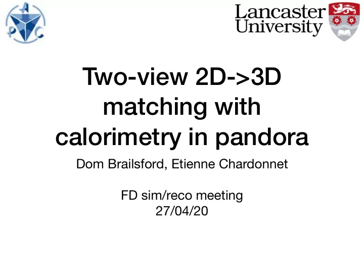
Two-view 2D->3D matching with calorimetry in pandora Dom Brailsford, Etienne Chardonnet FD sim/reco meeting 27/04/20

2D->3D matching • 2D->3D matching takes 2D clusters (e.g. from each wire view) and matching them across views to make 3D objects 
 • Pandora’s main 2D->3D matching algorithm requires a cluster in three distinct views to function • Combining positions from clusters in two of the views infers a position in the third view. A pseudo chi2 is calculated for inferred vs actual positions on the cluster 
 • This is problematic for any detector technology which only has two views (e.g. the CRP-based dual-phase LArTPCs) 2

*Resampling method suggested by Andy** **Suggested to Andy by Tom Junk Two-view 2D->3D matching • We are exploring how calorimetry could enhance two-view 2D->3D matching 
 • Exploratory algorithm details: 1. Make every pairwise comparison of 2D 400 450 500 550 600 V view 2300 clusters in the two views 2200 2. Find the region that the two clusters Time 2100 overlap each other in time 2000 2D cluster 1900 3. For that overlap region, produce fractional 1800 profiles of charge for each cluster 1700 U view 4. Downsample* the two charge profiles so 2300 that they are coarse and equally binned 2200 Time 2100 5. Calculate the charge profiles’ correlation 2000 2D cluster coe ffi cient and corresponding p-value (p- 1900 value calculation on next slide) 1800 550 600 650 700 750 • All plots are taken from custom samples made in ProtoDUNE dual-phase, but all details are directly relevant for the DUNE far detector, both single-phase and dual-phase 3


 
 
 Correlation coefficient’s p- value • For uncorrelated bivariate normal distribution pairs, the correlation coe ffi cient follows a Student t-distribution with n-2 degrees of freedom • The t-value is 
 • P-value is calculated by integrating the t-distribution above the calculated t value (a one tailed test) • H0: r==0 • H1: r>0 • The t-distribution supposedly approximately holds for non-gaussian variables, provided the sample sizes are large enough. I’ll revisit this in a few slides 4

Resampled fractional charge profiles (di-muon sample) Fractional value (no units) Fractional value (no units) 0.04 0.04 r: 0.142 r: 0.804 U cluster U cluster 0.035 p-value: 0.062 p-value: 7e-17 0.035 V cluster V cluster 0.03 0.03 0.025 0.025 0.02 0.02 0.015 0.015 0.01 0.01 0.005 0.005 0 0 10 20 30 40 50 5 10 15 20 25 30 35 40 45 50 x (cm) x (cm) Fractional value (no units) Fractional value (no units) 0.03 U cluster 0.04 U cluster 0.025 V cluster 0.035 V cluster 0.03 0.02 0.025 0.015 0.02 0.015 0.01 0.01 r: 0.821 r: 0.161 0.005 0.005 p-value: 1e-24 p-value: 0.119 10 20 30 40 50 60 70 80 5 10 15 20 25 30 35 40 45 50 5 x (cm) x (cm)

Further 2D->3D matching exploration • We can do a little bit more and try to correlate local regions of the profiles 
 • Once the resampled fractional charge profiles have been constructed • Slide a fixed-length window of N bins across the equally- binned charge profiles • Repeatedly calculate correlation coe ffi cient and p-value as the window slides across the profiles • For each p-value calculation, calculate a ‘matching score’ • Score == 1-p 6

Sliding window scores (same di-muon event) Matching score 1 Matching score 1 0.9 0.9 0.8 0.8 0.7 0.6 0.7 0.5 0.6 0.4 0.3 0.5 0 10 20 30 40 50 0 10 20 30 40 50 X (in cm) X (in cm) Matching score Matching score 1 1 0.9 0.9 0.8 0.7 0.8 0.6 0.7 0.5 0.4 0.6 0.3 0.5 0.2 0 10 20 30 40 50 60 70 80 90 0 10 20 30 40 50 X (in cm) X (in cm) 7

Resampled fractional charge profiles (1mu1p sample) Fractional value (no units) Fractional value (no units) 0.045 0.08 r: 0.778 r: 0.449 U cluster 0.04 p-value: 6e-16 p-value: 0.010 0.07 V cluster 0.035 0.06 0.03 0.05 0.025 0.04 0.02 0.03 0.015 U cluster 0.02 0.01 V cluster 0.01 0.005 0 0 10 20 30 40 50 10 20 30 40 50 x (cm) x (cm) Fractional value (no units) Fractional value (no units) 0.1 0.08 0.09 0.07 0.08 0.07 0.06 0.06 0.05 r: 0.781 0.05 0.04 r: 0.995 p-value: 0.001 0.04 0.03 p-value: -6.9e-10 U cluster U cluster 0.03 0.02 0.02 V cluster V cluster 0.01 0.01 10 20 30 40 50 10 20 30 40 50 60 70 8 x (cm) x (cm)

Sliding window scores (1mu1p event) Matching score 1 1 Matching score 0.9 0.8 0.8 0.6 0.7 0.4 0.6 0.2 0.5 0 10 20 30 40 50 60 0 10 20 30 40 50 60 X (in cm) X (in cm) Matching score Matching score 1 1 0.9 0.8 0.8 0.6 0.7 0.4 0.6 0.2 0.5 0 10 20 30 40 50 0 10 20 30 40 50 60 70 X (in cm) X (in cm) 9

Toy study 0.22 Correlated 0.2 fake profile 0.18 • Revisiting the student t-distribution 0.16 assumption 
 0.14 • Produce 10000 fake fractional charge 0.12 profiles 0.1 • Fill 3 histograms with landau throws, 0.08 smeared with a gaussian • Two hists. are filled with the same 0 1 2 3 4 5 6 7 8 9 10 landau values but smeared separately • Third hist filled with separate landau 0.22 values Uncorrelated 0.2 • Each bin is filled N times with distinct fake profile 0.18 throws to mimic the downsampling • Calculate correlation coe ffi cient and p- 0.16 value 0.14 0.12 • Landau (315, 13) • Gaus (1,0.1) 0.1 • N hist bins == 30 0.08 • N samples per bin == 5 0 1 2 3 4 5 6 7 8 9 10 10

No. universes 5000 Toy study 4000 3000 2000 • Top plot shows correlation coe ffi cient for the 10,000 1000 universes 0 • Black: correlated 1 0.8 0.6 0.4 0.2 0 0.2 0.4 0.6 0.8 1 − − − − − Correlation coefficient distributions No. universes 4 10 • Red: uncorrelated distributions 3 10 • Bottom plot shows corresponding p-values 2 10 • The red distribution 10 should be flat, but it is not 1 0 0.2 0.4 0.6 0.8 1 p-value 11

P-value vs r (t-distribution) 1 240 p 220 200 0.8 180 160 0.6 140 120 100 0.4 80 60 0.2 40 20 0 0 1 0.8 0.6 0.4 0.2 0 0.2 0.4 0.6 0.8 1 − − − − − r 12

No. universes 5000 Toy study 4000 3000 • Instead, calculate the p-value using permutation tests 2000 • Randomly shu ffl e the bins 1000 for one distribution in a comparison and 0 1 0.8 0.6 0.4 0.2 0 0.2 0.4 0.6 0.8 1 − − − − − recalculate r Correlation coefficient • P-value == fraction of No. universes 4 10 times you measure an r that is more extreme than 3 10 your original r measurement 2 10 • Top plot shows correlation coe ffi cient (same as previous 10 slide) • Bottom plot shows 1 corresponding p-value 0 0.2 0.4 0.6 0.8 1 13 p-value

p-value vs r (permutation test) 1 p 60 0.8 50 0.6 40 30 0.4 20 0.2 10 0 0 1 0.8 0.6 0.4 0.2 0 0.2 0.4 0.6 0.8 1 − − − − − r 14

Future and summary • Pandora’s main 2D->3D matching algorithm requires three views to operate • Not usable by detectors with two views, such as the CRP-based dual-phase LArTPCs • We are exploring the use of calorimetry in a new 2D->3D matching algorithm, suitable for two-view LArTPCs • The new matching algorithm tries to correlate the energy depositions between the two views to match clusters • So far, the calorimetry-based checks seem to do a good job of separating matching clusters vs non-matching clusters • While the t-test based p-value shows strong separation power, it is not a robust p-value, statistically speaking. Swapping to a permutation- test based p-value would rectify the robustness 15

Backup 16

*resampling suggested by Andy** **suggested to Andy by Tom Junk New two view matching alg • Overall aim is to 3D match 2D clusters by correlating the charge depositions in the clusters common transverse (time) overlap region 
 • Recipe (part 1) * • Collect candidate matching cluster hits that lie in the overlap region • Create cumulative distribution for each cluster’s overlap • Smooth the cumulative distribution using linear/quadratic/cubic interpolation. We are currently using linear interpolation due to quadratic/cubic instability in some regions of the distributions • Resample the two smoothed cumulative distributions such that they have coarser, equal binning. The current scheme downsamples to 1/5th the number of hits in the sparser cumulative distribution • Di ff erentiate the two resampled cumulative distributions to produce two equally binned fractional charge profiles • Calculate the correlation coe ffi cient and corresponding p-value between the two distributions 17

How binning alters r (toy study) No. universes No. universes 5000 2500 N. profile bins: 30 N. profile bins: 30 4000 N. samples ber bin: 1 N. samples ber bin: 5 2000 3000 1500 2000 1000 1000 500 0 0 − 1 − 0.8 − 0.6 − 0.4 − 0.2 0 0.2 0.4 0.6 0.8 1 − 1 − 0.8 − 0.6 − 0.4 − 0.2 0 0.2 0.4 0.6 0.8 1 Correlation coefficient Correlation coefficient 5000 No. universes No. universes 8000 N. profile bins: 150 N. profile bins: 150 7000 4000 N. samples ber bin: 1 N. samples ber bin: 5 6000 5000 3000 4000 2000 3000 2000 1000 1000 0 0 − 1 − 0.8 − 0.6 − 0.4 − 0.2 0 0.2 0.4 0.6 0.8 1 − 1 − 0.8 − 0.6 − 0.4 − 0.2 0 0.2 0.4 0.6 0.8 1 18 Correlation coefficient Correlation coefficient

Before 19

Now 20

Now 21