[PPT] - Rare events: models and simulations Josselin Garnier (Universit e PowerPoint Presentation

SLIDE 1

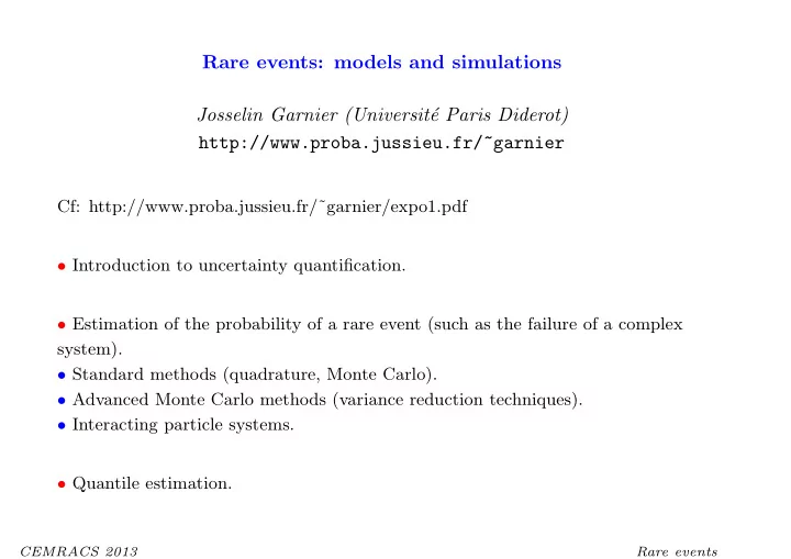
Rare events: models and simulations Josselin Garnier (Universit´ e Paris Diderot) http://www.proba.jussieu.fr/~garnier

Cf: http://www.proba.jussieu.fr/˜garnier/expo1.pdf

Introduction to uncertainty quantification.
Estimation of the probability of a rare event (such as the failure of a complex

system).

Standard methods (quadrature, Monte Carlo).
Advanced Monte Carlo methods (variance reduction techniques).
Interacting particle systems.
Quantile estimation.

CEMRACS 2013 Rare events

SLIDE 2

Uncertainty quantification

General problem:
How can we model the uncertainties in physical and numerical models ?
How can we estimate (quantify) the variability of the output of a code or an

experiment as a function of the variability of the input parameters ?

How can we estimate quantify the sensitivity or the variability of the output of a

code or an experiment with respect to one particular parameter ?

CEMRACS 2013 Rare events

SLIDE 3

✬ ✫ ✩ ✪

Step 1 Quantification

f the sources
f uncertainty

Law of X

✲ ✬ ✫ ✩ ✪

Step 0 Definition of the model Y = f(X) Input X Output Y

✲ ✬ ✫ ✩ ✪

Step 2 Uncertainty propagation Central trends Rare events Quantile

✻ ✤ ✣ ✜ ✢

Step 3 Sensitivity analysis Local variational approach Global stochastic approach

✛

CEMRACS 2013 Rare events

SLIDE 4

Uncertainty propagation

Context: numerical code (black box) or experiment

Y = f(X) with Y = output X = random input parameters, with known distribution (with pdf p(x)) P(X ∈ A) =

A

p(x)dx for any A ∈ B(Rd) f = deterministic function Rd → R (computationally expensive).

Goal: estimation of a quantity of the form

E[g(Y )] with an “error bar” and the minimal number of simulations. Examples (for a real-valued output Y ):

g(y) = y → mean of Y , i.e. E[Y ]
g(y) = y2 → variance of Y , i.e. Var(Y ) = E[(Y − E[Y ])2] = E[Y 2] − E[Y ]2
g(y) = 1[a,∞)(y) → probability P(Y ≥ a).

CEMRACS 2013 Rare events

SLIDE 5

Analytic method

The quantity to be estimated is a d-dimensional integral:

I = E[g(Y )] = E[h(X)] =

Rd h(x)p(x)dx

where p(x) is the pdf of X and h(x) = g(f(x)).

In simple cases (when the pdf p and the function h have explicit expressions),
ne can sometimes evaluate the integral exactly (exceptional situation).

CEMRACS 2013 Rare events

SLIDE 6

Quadrature method

The quantity to be estimated is a d-dimensional integral:

I = E[g(Y )] = E[h(X)] =

Rd h(x)p(x)dx

where p(x) is the pdf of X and h(x) = g(f(x)).

If p(x) = d

i=1 p0(xi), then it is possible to apply Gaussian quadrature with a

tensorized grid with nd points: ˆ I =

n

j1=1

· · ·

n

jd=1

ρj1 · · · ρjdh(ξj1, . . . , ξjd) with the weights (ρj)j=1,...,n and the points (ξj)j=1,...,n associated to the quadrature with weighting function p0.

There exist quadrature methods with sparse grids (cf Smolyak).
Quadrature methods are efficient when:
the function x → h(x) is smooth (and not only f),
the dimension d is “small” (even with sparse grids).

They require many calls.

CEMRACS 2013 Rare events

SLIDE 7

Monte Carlo method

Principle: replace the statistical expectation E[g(Y )] by an empirical mean.

CEMRACS 2013 Rare events

SLIDE 8

Monte Carlo method: “head and tail” model

A code gives a real-valued output Y = f(X). For a given a we want to estimate P = P(f(X) ≥ a)

Monte Carlo method:

1) n simulations are carried out with n independent realizations X1, . . . , Xn (with the distribution of X). 2) let us define Zk = 1[a,∞)(f(Xk)) =    1 if f(Xk) ≥ a (head) if f(Xk) < a (tail)

Intuition: when n is large, the empirical proportion of “1”s is close to P

Z1 + · · · + Zn n ≃ P Therefore the empirical proportion of “1”s can be used to estimate P.

Empirical estimator of P:

ˆ Pn := 1 n

n

k=1

Zk

CEMRACS 2013 Rare events

SLIDE 9

Empirical estimator of P:

ˆ Pn := 1 n

n

k=1

Zk

The estimator is unbiased:

E

ˆ

Pn

= E
1

n

k=1

Zk

= 1

n

k=1

E[Zk] = E[Z1]= P

The law of large numbers shows that the estimator is convergent:

ˆ Pn = 1 n

n

k=1

Zk

n→∞

− → E[Z1] = P because the variables Zk are independent and identically distributed (i.i.d.).

Result (law of large numbers): Let (Zn)n∈N∗ be a sequence of i.i.d. random
variables. If E[|Z1|] < ∞, then

1 n

n

k=1

Zk

n→∞

− → m with probability 1, with m = E[Z1] “The empirical mean converges to the statistical mean”.

CEMRACS 2013 Rare events

SLIDE 10

Error analysis: we want to quantify the fluctuations of ˆ Pn around P.

Variance calculation:

Var[ ˆ Pn] = E

( ˆ

Pn − P)2 (mean square error) = E n

k=1

Zk − P n 2 =

n

k=1

E Zk − P n 2 = 1 n2

n

k=1

E

(Zk − P)2

= 1 nE

(Z1 − P)2

= 1 n

E
Z2

1

− P 2

= 1 n(P − P 2)

The relative error is therefore:

Error =

Var( ˆ

Pn) E[ ˆ Pn] =

Var( ˆ

Pn) P = 1 √n 1 P − 1 1/2

CEMRACS 2013 Rare events

SLIDE 11

Confidence intervals

Question: The estimator ˆ

Pn gives an approximate value of P, all the better as n is larger. How to quantify the error ?

Answer: We build a confidence interval at the level 0.95, i.e. an empirical

interval [ˆ an,ˆ bn] such that P

P ∈ [ˆ

an,ˆ bn]

≥ 0.95

Construction based on the De Moivre theorem: P

ˆ

Pn − P

< c

√ P − P 2 √n

n→∞

− → 2 √ 2π c e−x2/2dx The right member is 0.05 if c = 1.96. Therefore P

P ∈
ˆ

Pn − 1.96 √ P − P 2 √n , ˆ Pn + 1.96 √ P − P 2 √n

≃ 0.95
Result (central limit theorem): Let (Zn)n∈N∗ be a sequence of i.i.d. random
variables. If E[Z2

1] < ∞, then

√n 1 n

n

k=1

Zk − m

n→∞

− → N(0, σ2) in distribution where m = E[Z1] and σ2 = Var(Z1). “For large n, the error 1

n

k=1 Zk − m has Gaussian distribution N(0, σ2/n).”

CEMRACS 2013 Rare events

SLIDE 12

P

P ∈
ˆ

Pn − 1.96 √ P − P 2 √n , ˆ Pn + 1.96 √ P − P 2 √n

≃ 0.95

The unknown parameter P is still in the bounds of the interval ! Two solutions:

P ∈ [0, 1], therefore

√ P − P 2 < 1/2 and P

P ∈
ˆ

Pn − 0.98 1 √n, ˆ Pn + 0.98 1 √n

≥ 0.95
asymptotically, we can replace P in the bounds by ˆ

Pn (OK if nP > 10 and n(1 − P) > 10): P  P ∈   ˆ Pn − 1.96

ˆ

Pn − ˆ P 2

n

√n , ˆ Pn + 1.96

ˆ

Pn − ˆ P 2

n

√n     ≃ 0.95 Conclusion: There is no bounded interval of R that contains P with probability

ne. There are bounded intervals (called confidence intervals) that contain P with

probability close to one (chosen by the user).

CEMRACS 2013 Rare events

SLIDE 13

Monte Carlo estimation: black box model

Black box model (numerical code)

Y = f(X) We want to estimate I = E[g(Y )], for some function g : R → R.

Empirical estimator:
In = 1

n

k=1

g(f(Xk)) where (Xk)k=1,...,n is a n-sample of X. This is the empirical mean of a sequence of i.i.d. random variables.

The estimator

In is unbiased: E[ In] = I.

The law of large numbers gives the convergence of the estimator:
In

n→∞

− → I with probability 1

CEMRACS 2013 Rare events

SLIDE 14

Error:

Var( In) = 1 nVar(g(Y )) Proof: the variance of a sum of i.i.d. random variables if the sum of the variances.

Asymptotic confidence interval:

P

I ∈
In − 1.96 ˆ

σn √n, In + 1.96 ˆ σn √n

≃ 0.95

where ˆ σn =

1

n

k=1

g(f(Xk))2 − I2

n

1/2

Advantages of the MC method:

1) no regularity condition for f, g (condition: E[g(f(X))2] < ∞). 2) convergence rate 1/√n in any dimension. 3) can be applied for any quantity that can be expressed as an expectation.

One needs to simulate samples of X.

CEMRACS 2013 Rare events

SLIDE 15

Simulation of random variables

How do we generate random numbers with a computer ? There is nothing

random in a computer !

Strategy:
find a pseudo random number generator that can generate a sequence of numbers

that behave like independant copies of a random variable with uniform distribution over (0, 1).

use deterministic transforms to generate numbers with any prescribed

distribution using only the uniform pseudo random number generator.

CEMRACS 2013 Rare events

SLIDE 16

Pseudo random number generator

A 32-bit multiplicative congruential generator: xn+1 = axn mod b, with a = 75, b = 231 − 1, and some integer x0. This gives a sequence of integer numbers in {0, 1, ..., 231 − 2}. The sequence un = xn/(231 − 1) gives a “quasi-real” number between 0 and 1. Note: the sequence is periodic, with period 231 − 1. This is the generator mcg16807 of matlab (used in early versions). Today: matlab uses mt19937ar (the period is 219937 − 1).

CEMRACS 2013 Rare events

SLIDE 17

Inversion method.

A little bit of theory: Result: Let X be a real random variable with the cumulative distribution function (cdf) F(x): F(x) = P(X ≤ x) = x

−∞

p(y)dy Let U be a random variable with the distribution U(0, 1). If F is one-to-one, then X and F −1(U) have the same distribution. Proof: Set Y = F −1(U). P(Y ≤ x) = P(F −1(U) ≤ x) = P(U ≤ F(x)) = F(x) , which shows that the cdf of Y is F.

CEMRACS 2013 Rare events

SLIDE 18

Extension: Let F be a cdf. The generalized inverse of F is F −1 : (0, 1) → R

defined by: F −1(u) := inf Au, where Au := {x ∈ R such that F(x) ≥ u} The generalized inverse always exists because, for any u ∈ (0, 1): (i) limx→+∞ F(x) = 1, therefore Au = ∅. (ii) limx→−∞ F(x) = 0, therefore Au is bounded from below. Result: Let X be a random variable with the cdf F(x). Let U be a random variable with the distribution U(0, 1). Then X and F −1(U) have the same distribution.

CEMRACS 2013 Rare events

SLIDE 19

Example. Let us write a simulator of an exponential random variable:

p(x) = e−x1[0,∞)(x) Its cdf is F(x) =    if x < 0, x

0 e−ydy = 1 − e−x

if x ≥ 0 whose reciprocal is: F −1(u) = − ln(1 − u) . Therefore if U is a uniform random variable on [0, 1], then the random variable X := − ln(1 − U) obeys the exponential distribution. Moreover, U and 1 − U have the same distribution, therefore − ln(U) also obeys the exponential distribution.

CEMRACS 2013 Rare events

SLIDE 20

Simulation of Gaussian random variables.

The inversion method requires the knowledge of the reciprocal cdf F −1. We do not always have the explicit expression of this reciprocal function. An important example is the Gaussian distribution such that F(x) =

1 √ 2π

x

−∞ e−s2/2ds for x ∈ R.

Box-Muller algorithm: Let U1, U2 two independent random variables with uniform distribution over [0, 1]. If X = (−2 ln U1)1/2 cos(2πU2) Y = (−2 ln U1)1/2 sin(2πU2) then the random variables X and Y are independent and distributed according to N(0, 1). Proof: for any test function f : Rd → R, write E[f(X, Y )] as a two-dimensional integral and use polar coordinates.

CEMRACS 2013 Rare events

SLIDE 21

Rejection method for uniform distributions.
Goal: build a generator of a random variable with uniform distribution over

D ⊂ Rd.

Preliminary: Find a rectangular domain B such that D ⊂ B.
Algorithm:

Sample M1, M2, . . . independent and identically distributed with the uniform distribution over B, until the first time T when Mi ∈ D.

Result: MT is a random variable with the uniform distribution over D.
Warning: the distribution of MT is not the distribution of M1, because T is

random ! The time T obeys a geometric distribution with mean |B|/|D| (→ it is better to look for the smallest domain B).

CEMRACS 2013 Rare events

SLIDE 22

Rejection method for continuous distributions.
Goal: build a generator of a random variable with pdf p(x).
Preliminary: find a pdf q(x) such that we know a generator of a random variable

with pdf q(x) and we know C ≥ 1 such that p(x) ≤ Cq(x) for all x ∈ Rd.

Algorithm:

Sample X1, X2, . . . with pdf q(x) and U1, U2, . . . with distribution U(0, 1) until the first time T when Uk < p(Xk)/[Cq(Xk)].

Result: XT is a random variable with the pdf p(x).

The time T obeys a geometric distribution with mean C.

CEMRACS 2013 Rare events

SLIDE 23

Proof: for any Borel set A: P(XT ∈ A) =

∞

k=1

P(Xk ∈ A, T = k) =

∞

k=1

P

Xk ∈ A, Uk <

p(Xk) Cq(Xk), Uk−1 ≥ p(Xk−1) Cq(Xk−1), . . . , U1 ≥ p(X1) Cq(X1)

=

∞

k=1

P

X1 ∈ A, U1 <

p(X1) Cq(X1)

P
U1 ≥

p(X1) Cq(X1) k−1 = P

X1 ∈ A, U1 <

p(X1) Cq(X1))

P

U1 <

p(X1) Cq(X1)

=

EX

1X1∈AEU[1U1< p(X1)

Cq(X1) ]

EX
EU[1U1< p(X1)

Cq(X1) ]

=

EX

1X1∈A

p(X1) Cq(X1)

EX

p(X1)

Cq(X1)

=
1x∈A

p(x) Cq(x) q(x)dx

p(x)

Cq(x) q(x)dx

=

1x∈Ap(x)dx

CEMRACS 2013 Rare events

SLIDE 24

Estimation of the probability of a rare event

We look for an estimator for

P = P(f(X) ≥ a) where a is large (so that P ≪ 1).

Possible by Monte Carlo:

ˆ Pn = 1 n

n

k=1

1f(Xk)≥a where (Xk)k=1,...,n is a n-sample of X. Relative error: E[( ˆ Pn − P)2]1/2 P = 1 √n Var(1f(X)≥a)1/2 P = 1 √n √ 1 − P √ P

P ≪1

≃ 1 √ nP ֒ → We need nP > 1 so that the relative error is smaller than 1 (not surprising) ! ֒ → We need variance reduction techniques.

CEMRACS 2013 Rare events

SLIDE 25

Uncertainty propagation by metamodels

The complex code/experiment f is replaced by a metamodel (reduced model) fr and one of the previous techniques is applied with fr (analytic, quadrature, Monte Carlo). → It is possible to call many times the metamodel. → The choice of the metamodel is critical. → The error control is not simple.

CEMRACS 2013 Rare events

SLIDE 26

Taylor expansions

We approximate the output Y = f(X) by a Taylor series expansion Yr = fr(X).
Example:
We want to estimate E[Y ] and Var(Y ) for Y = f(X) with Xi uncorrelated,

E[Xi] = µi and Var(Xi) = σ2

i known, σ2 i small.

We approximate Y = f(X) by Yr = fr(X) = f(µ) + ∇f(µ) · (X − µ). We find:

E[Y ] ≃ E[Yr] = f(µ), Var(Y ) ≃ Var(Yr) =

d

i=1

∂xif(µ)2σ2

i

We just need to compute f(µ) and ∇f(µ) (evaluation of the gradient by finite differences, about d + 1 calls to f).

Rapid, analytic, allows to evaluate approximately central trends of the output

(mean, variance).

Suitable for small variations of the input parameters and a smooth model (that

can be linearized).

Local approach. In general, no error control.

CEMRACS 2013 Rare events

SLIDE 27

Reliability method for estimation of the probability of a rare event: P = P(f(X) ≥ a) = P(X ∈ F) =

F

p(x)dx, F = {x ∈ Rd, f(x) ≥ a}

The FORM-SORM method is analytic but approximate, without control error.
The Xi are assumed to be independent and with Gaussian distribution with

mean zero and variance one (or we use an isoprobabilist transform to deal with this situation): p(x) =

1 (2π)d/2 exp(− |x|2 2 ).

One gets by optimization (with contraint) the “design point” xa (the most

probable failure point), i.e. xa = argmin{x2 s.t. f(x) ≥ a}.

One approximates the failure surface {x ∈ Rd, f(x) = a} by a smooth surface ˆ

F that allows for an analytic calculation ˆ P =

ˆ

F p(x)dx:

a quadratic form for SORM

(and then ˆ P = 1

2erfc

|xa|

√ 2

),
a hyperplane for FORM

(and then ˆ P = Breitung’s formula). Cf: O. Ditlevsen et H.O. Madsen, Structural reliability methods, Wiley, 1996.

2 4 6 1 2 3 4 5 xa f(x)>a f(x)<a FORM SORM

CEMRACS 2013 Rare events

SLIDE 28

Variance reduction techniques

Goal: reduce the variance of the Monte Carlo estimator: E

(ˆ

In − I)2 = 1 nVar(h(X)) where h(x) = g(f(x)), I = E[h(X)], In = 1

n

k=1 h(Xk).

The methods
Importance sampling
Control variates
Antithetic variables
Stratification

reduce the constant without changing 1/n, stay close to the Monte Carlo method (parallelizable).

The methods
Quasi-Monte Carlo

aim at changing 1/n.

The methods
Interacting particle systems (genetic algorithms, subset sampling,. . .)

are more different from Monte Carlo (sequential).

CEMRACS 2013 Rare events

SLIDE 29

Importance sampling

The goal is to estimate I = E[h(X)] for X a random vector and h(x) = g(f(x))

a deterministic function.

Observation: the representation of I as an expectation is not unique. If X has

the pdf p(x): I = Ep[h(X)] =

h(x)p(x)dx =

h(x)p(x) q(x) q(x)dx = Eq h(X)p(X) q(X)

The choice of the pdf q depends on the user.
Idea: when we know that h(X) is sensitive to certain values of X, instead of

sampling Xk with the original pdf p(x) of X, a biased pdf q(x) is used that makes more likely the “important” realizations.

Using the representation

I = Ep[h(X)] = Eq

h(X)p(X)

q(X)

we can propose the estimator:

ˆ In = 1 n

n

k=1

h(Xk)p(Xk) q(Xk) where (Xk)k=1,...,n is a n-sample with the distribution with pdf q.

CEMRACS 2013 Rare events

SLIDE 30

The estimator is unbiased:

Eq[ In] = 1 n

n

k=1

Eq

h(Xk)p

q (Xk)

= Eq
h(X)p

q (X)

=
h(x)p

q (x)q(x)dx =

h(x)p(x)dx = Ep
h(X)
= I
The estimator is convergent:

ˆ In = 1 n

n

k=1

h(Xk)p(Xk) q(Xk)

n→∞

− → Eq

h(X)p(X)

q(X)

= Ep
h(X)
= I
The variance of the estimator is:

Var(ˆ In) = 1 nVarq

h(X)p(X)

q(X)

= 1

n

Ep
h(X)2 p(X)

q(X)

− Ep [h(X)]2
By a judicious choice of q the variance can be dramatically reduced.
Critical points: it is necessary to know the likelihood ratio p(x)

q(x) and to know how to simulate X with the pdf q.

CEMRACS 2013 Rare events

SLIDE 31

Optimal importance sampling.

The best importance distribution is the one that minimizes the variance Var(ˆ In). It is the solution of the minimization problem: find the pdf q(x) minimizing Ep

h(X)2 p(X)

q(X)

=
h(x)2 p2(x)

q(x) dx Solution (when h is nonnegative-valued): qopt(x) = h(x)p(x)

h(x′)p(x′)dx′

We then find Var(ˆ In) = 1 n

Ep
h(X)2 p(X)

qopt(X)

− Ep [h(X)]2
= 0 !

Pratically: the denominator of qopt(x) is the desired quantity E[h(X)], which is

unknown. Therefore the optimal importance distribution is unknown (principle for

an adaptive method).

CEMRACS 2013 Rare events

SLIDE 32

Example: We want to estimate

I = E[h(X)] with X ∼ N(0, 1) and h(x) = 1[4,∞)(x). I = 1 √ 2π ∞

−∞

1[4,∞)(x)e− x2

2 dx = 1

2erfc 4 √ 2

≃ 3.17 10−5

Monte Carlo: With a sample (Xk)k=1,...,n with the original distribution N(0, 1). ˆ In = 1 n

n

k=1

1Xk≥4, Xk ∼ N(0, 1) We have Var(ˆ In) = 1

n3.17 10−5.

Importance sampling: With a sample (Xk)k=1,...,n with the distribution N(4, 1). ˆ In = 1 n

n

k=1

1Xk≥4 e−

X2 k 2

e− (Xk−4)2

2

= 1 n

n

k=1

1Xk≥4e−4Xk+8, Xk ∼ N(4, 1) We have Var(ˆ In) = 1

n5.53 10−8.

The IS method needs 1000 times less simulations to reach the same precision as MC !

CEMRACS 2013 Rare events

SLIDE 33

Warning: we should not bias too much. Importance sampling: With a sample (Xk)k=1,...,n with the distribution N(µ, 1). ˆ In = 1 n

n

k=1

1Xk≥4 e−

X2 k 2

e− (Xk−µ)2

2

= 1 n

n

k=1

1Xk≥4e−µXk+ µ2

2 ,

Xk ∼ N(µ, 1) We have Var(ˆ In) = 1

n eµ2 2 erfc

4+µ

√ 2

− 1

nI2, which gives the normalized relative

error √nE[(ˆ In − I)2]1/2/I :

2 4 6 8 10 10

1

10

2

10

3

µ n1/2 relative error

If the bias is too large, the fluctuations of the likelihood ratios become large.

CEMRACS 2013 Rare events

SLIDE 34

Example: we want to estimate

I = E[h(X)] with X ∼ N(0, 1) and h(x) = exp(x). I = 1 √ 2π

exe− x2

2 dx = e 1 2

The large values of X are important. Importance sampling: With a sample (Xk)k=1,...,n with the distribution N(µ, 1), µ > 0. ˆ In = 1 n

n

k=1

h(Xk) e− [Xk]2

2

e− [Xk−µ]2

2

= 1 N

n

k=1

h(Xk)e−µXk+ µ2

2

Var(ˆ In) = 1 n

eµ2−2µ+2 − e1

Monte Carlo µ = 0: Var(ˆ In) = 1

n

e2 − e1

Optimal importance sampling µ = 1: Var(ˆ In) = 0.

CEMRACS 2013 Rare events

SLIDE 35

Control variates

The goal is to estimate I = E[h(X)] for X a random vector and h(x) = g(f(x))

a deterministic function.

Assume that we have a reduced model fr(X).
Importance sampling method: first we evaluate (we approximate) the optimal

density qopt,r(x) = g(fr(x))p(x)

Ir

, with Ir =

g(fr(x))p(x)dx, then we use it as a

biased density for estimating I (dangerous, use conservative version).

Control variates method:

We denore h(x) = g(f(x)), hr(x) = g(fr(x)). We assume that we know Ir = E[hr(X)]. By considering the representation I = E[h(X)] = Ir + E[h(X) − hr(X)] we propose the estimator: ˆ In = Ir + 1 n

n

k=1

h(Xk) − hr(Xk), where (Xk)k=1,...,n is a n-sample (with the pdf p).

CEMRACS 2013 Rare events

SLIDE 36

Estimator:

ˆ In = Ir + 1 n

n

k=1

h(Xk) − hr(Xk)

The estimator is unbiased:

E

In
=

Ir + 1 n

n

k=1

E

h(Xk) − hr(Xk)
= Ir + E[h(X)] − E[hr(X)]

= Ir + E[h(X)] − Ir = I

The estimator is convergent:
In

n→∞

− → Ir + E

h(X) − hr(X)
= I
The variance of the estimator is:

Var( In) = 1 nVar

h(X) − hr(X)
֒

→ The use of a reduced model can reduce the variance.

CEMRACS 2013 Rare events

SLIDE 37

Example: we want to estimate

I = E[h(X)] with X ∼ U(0, 1), h(x) = exp(x). Result: I = e − 1 ≃ 1.72. Monte Carlo. ˆ In = 1 n

n

k=1

exp[Xk] Variance of the MC estimator= 1

n(2e − 1) ≃ 1 n4.44.

Control variates. Reduced model: hr(x) = 1 + x (here Ir = 3

2). CV estimator:

ˆ In = Ir + 1 n

n

k=1

{exp[Xk] − 1 − Xk} Variance of the CV estimator = 1

n(3e − e2 2 − 53 12) ≃ 1 n0.044.

The CV method needs 100 times less simulations to reach the same precision as MC !

CEMRACS 2013 Rare events

SLIDE 38

Application: estimation of

I = E[g(f(X))] We have a reduced model fr of the full code f. The ratio between the computational cost of one call of f and one call of fr is q > 1. Estimator ˆ In = 1 nr

nr

k=1

hr( ˜ Xk) + 1 n

n

k=1

h(Xk) − hr(Xk) with nr > n, h(x) = g(f(x)), hr(x) = g(fr(x)). Allocation between calls to the full code and calls to the reduced model can be

ptimized with the contraint nr/q + n(1 + 1/q) = ntot.

Classical trade-off between approximation error and estimation error. Used when f(X) is the solution of an ODE or PDE with fine grid, while fr(X) is the solution obtained with a coarse grid (MultiLevel Monte Carlo).

CEMRACS 2013 Rare events

SLIDE 39

Not very useful for the estimation of the probability of a rare event.

Example: we want to estimate I = P(f(X) ≥ 2.7) with X ∼ U(0, 1), f(x) = exp(x). Result: I = 1 − ln(2.7) ≃ 6.7 10−3. The reduced model fr(x) = 1 + x is here useless. The reduced model should be good in the important region.

CEMRACS 2013 Rare events

SLIDE 40

Stratification

Principle: The sample (Xk)k=1,...,n is enforced to obey theoretical distributions in some “strata”. Method used in polls (representative sample). Here: we want to estimate E[g(f(X))], X with values in D.

Two ingredients:

i) A partition of the state space D: D = m

i=1 Di. We know pi = P(X ∈ Di).

ii) Total probability formula: I = E[g(f(X))] =

m

i=1

E[g(f(X))|X ∈ Di]

J(i)

P(X ∈ Di)

pi
Estimation:

1) For all i = 1, . . . , m, Ii is estimated by Monte Carlo with ni simulations:

J(i)

ni = 1

ni

j=1

g(f(X(i)

j )),

X(i)

j

∼ L(X|X ∈ Di) 2) The estimator is

In =

m

i=1
J(i)

ni pi

CEMRACS 2013 Rare events

SLIDE 41

In =

m

i=1

pi J(i)

ni ,

J(i)

ni = 1

ni

j=1

g(f(X(i)

j )),

X(i)

j

∼ L(X|X ∈ Di) The total number of simulations is n = m

i=1 ni.

The estimator is unbiased, convergent and its variance is

Var

gn
S =

m

i=1

p2

i Var

J(i)

ni

=

m

i=1

p2

i

σ2

i

ni , with σ2

i = Var

g(f(X))|X ∈ Di
The user is free to choose the allocations ni (with the constraint m

i=1 ni = n).

Proportional stratification: ni = pin.
In =

m

i=1

pi ni

ni

j=1

g(f(X(i)

j )) = 1

n

m

i=1

ni

j=1

g(f(X(i)

j )),

X(i)

j

∼ L(X|X ∈ Di) Then Var

In
SP = 1

n

m

i=1

piσ2

i

We have: Var

In
MC = 1

nVar

g(f(X))
≥ 1

n

m

i=1

piσ2

i = Var

In
SP

CEMRACS 2013 Rare events

SLIDE 42

Proof: We have E[h(X)]2 =

m
i=1

piE[h(X)|X ∈ Di] 2 ≤

m
i=1

pi

m
i=1

piE[h(X)|X ∈ Di]2 =

m

i=1

piE[h(X)|X ∈ Di]2 Therefore

m

i=1

piσ2

i

=

m

i=1

pi

E[h(X)2|X ∈ Di] − E[h(X)|X ∈ Di]2

= E[h(X)2] −

m

i=1

piE[h(X)|X ∈ Di]2 ≤ E[h(X)2] − E[h(X)]2 = Var(h(X))

CEMRACS 2013 Rare events

SLIDE 43

However, the proportional allocation is not optimal !

The optimal allocation is the one that minimizes the variance

Var( In)S = m

i=1 p2 i σ2

i

ni .

It is the solution of the minimization problem: find (ni)i=1,...,m minimizing

m

i=1

p2

i

σ2

i

ni with the constraint

m

i=1

ni = n Solution (optimal allocation, obtained with Lagrange multiplier method): ni = n piσi m

l=1 plσl

The minimal variance is Var

In
SO = 1

n m

i=1

piσi 2 , We have: Var

In
SO ≤ Var
In
SP ≤ Var
In
MC

Practically: the σi’s are unknown, therefore the optimal allocation is unknown (principle of an adaptive method).

CEMRACS 2013 Rare events

SLIDE 44

Example: we want to estimate

E[g(f(X))] with X ∼ U(−1, 1), f(x) = exp(x) and g(y) = y. Result: E[f(X)] = sinh(1) ≃ 1.18. Monte Carlo. With a sample X1, ..., Xn with the distribution U(−1, 1)

In = 1

n

k=1

exp[Xk] Variance of the estimator = 1

n( 1 2 − e−2 2 ) ≃ 1 n0.43.

Proportional stratification. With a sample

X1, ..., Xn/2 with the distribution U(−1, 0),
Xn/2+1, ..., Xn with the distribution U(0, 1).
In = 1

n

n/2

k=1

exp[Xk] + 1 n

n

k=n/2+1

exp[Xk] = 1 n

n

k=1

exp[Xk] Variance of the PS estimator ≃ 1

n0.14.

The PS method needs 3 times less simulations to reach the same precision as MC.

CEMRACS 2013 Rare events

SLIDE 45

Nonproportional stratification. With a sample

X1, ..., Xn/4 with the distribution U(−1, 0),
Xn/4+1, ..., Xn with the distribution U(0, 1).
In = 2

n

n/4

k=1

exp[Xk] + 1 2n

n

k=n/4+1

exp[Xk] Variance of the estimator ≃ 1

n0.048.

The stratification method needs 9 times less simulations to reach the same precision as MC.

CEMRACS 2013 Rare events

SLIDE 46

Antithetic variables

We want to compute

I =

[0,1]d h(x)dx

Monte Carlo with a n-sample (X1, . . . , Xn) with the distribution U([0, 1]d): ˆ In = 1 n

n

k=1

h(Xk) E

(ˆ

In − I)2 = 1 nVar(h(X)) = 1 n

[0,1]d h2(x)dx − I2

We consider the representations

I =

[0,1]d h(1 − x)dx and I =
[0,1]d

h(x) + h(1 − x) 2 dx Monte Carlo with a n/2-sample (X1, . . . , Xn/2) with the distribution U([0, 1]d) : ˜ In = 1 n

n/2

k=1

h(Xk) + h(1 − Xk)

CEMRACS 2013 Rare events

SLIDE 47

Monte Carlo estimator with the sample

( ˜ X1, . . . , ˜ Xn) := (X1, . . . , Xn/2, 1 − X1, . . . , 1 − Xn/2) that is not i.i.d.: ˜ In = 1 n

n

k=1

h( ˜ Xk) The function f is called n times.

Error:

E

(˜

In − I)2 = 1 n

Var(h(X)) + Cov(h(X), h(1 − X))
=

1 n

[0,1]d h2(x) + h(x)h(1 − x)dx − 2I2

The variance is reduced if Cov(h(X), h(1 − X)) < 0. Sufficient condition: h is monotoneous.

Proof: If X, X′ i.i.d. [h(X) − h(X′)][−h(1 − X) + h(1 − X′)] ≥ 0 a.s. −2E

h(X)h(1 − X)
+ 2E
h(X)

2 ≥

CEMRACS 2013 Rare events

SLIDE 48

Example:

I = 1 1 1 + xdx Result: I = ln 2. Monte Carlo: ˆ In = 1 n

n

k=1

1 1 + Xk Var(ˆ In) = 1

n

1

0 (1 + x)−2dx − ln 22

= 1

n

1

2 − ln 22

≃ 1

n1.95 10−2.

Antithetic variables: ˜ In = 1 n

n/2

k=1

1 1 + Xk + 1 2 − Xk Var(˜ In) = 2

n

1

1

2(1+x) + 1 2(2−x)

2dx − ln 22 ≃ 1

n1.2 10−3.

The AV method requires 15 times less simulations than MC.

CEMRACS 2013 Rare events

SLIDE 49

More generally: one needs to find a pair (X, ˜

X) such that h(X) and h( ˜ X) have the same distribution and Cov(h(X), h( ˜ X)) < 0.

Monte Carlo with an i.i.d. sample ((X1, ˜

X1), . . . , (Xn/2, ˜ Xn/2)) : ˜ In = 1 n

n/2

k=1

h(Xk) + h( ˜ Xk) E

(˜

In − I)2 = 1 n

Var(h(X)) + Cov(h(X), h( ˜

X))

Recent application: computation of effective tensors in stochastic

homogenization (the effective tensor is the expectation of a functional of the solution of an elliptic PDE with random coefficients; antithetic pairs of the realizations of the composite medium are sampled; gain by a factor 3; in fact, better results with control variates; cf C. Le Bris, F. Legoll).

Not very useful for the estimation of probabilities of rare events.

CEMRACS 2013 Rare events

SLIDE 50

Low-discrepancy sequences (quasi Monte Carlo)

The sample (Xk)k=1,...,n is selected so as to fill the (random) gaps that appear

in a MC sample (for a uniform sampling of an hypercube).

This technique
can reduce the variance if h has good properties (bounded variation in the sense
f Hardy and Krause); the asymptotic variance can be of the form

Cd(log n)s(d)/n2,

can be applied in low-moderate dimension,
can be viewed as a compromise between quadrature and MC.
A few properties:
the error estimate is deterministic, but often not precise (Koksma-Hlawka

inequality),

the independence property is lost (→ it is not easy to add points),
the method is not adapted for the estimation of the probability of a rare event.

Cf lecture by G. Pag` es.

CEMRACS 2013 Rare events

SLIDE 51

Example: Monte Carlo sample.

0.1 0.2 0.3 0.4 0.5 0.6 0.7 0.8 0.9 1 0.1 0.2 0.3 0.4 0.5 0.6 0.7 0.8 0.9 1 0.1 0.2 0.3 0.4 0.5 0.6 0.7 0.8 0.9 1 0.1 0.2 0.3 0.4 0.5 0.6 0.7 0.8 0.9 1 0.1 0.2 0.3 0.4 0.5 0.6 0.7 0.8 0.9 1 0.1 0.2 0.3 0.4 0.5 0.6 0.7 0.8 0.9 1

n = 100 n = 1000 n = 10000

CEMRACS 2013 Rare events

SLIDE 52