Interacting particle systems for the analysis of rare events - PowerPoint PPT Presentation

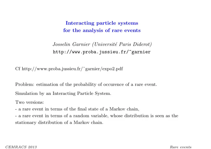
Interacting particle systems for the analysis of rare events Josselin Garnier (Universit´ e Paris Diderot) http://www.proba.jussieu.fr/~garnier Cf http://www.proba.jussieu.fr/˜garnier/expo2.pdf Problem: estimation of the probability of occurence of a rare event. Simulation by an Interacting Particle System. Two versions: - a rare event in terms of the final state of a Markov chain, - a rare event in terms of a random variable, whose distribution is seen as the stationary distribution of a Markov chain. CEMRACS 2013 Rare events

Rare events • Description of the system: Let E be a measurable space. − ( X p ) 0 ≤ p ≤ M : a E -valued Markov chain: P ( X p ∈ A | X p − 1 = x p − 1 , . . . , X 0 = x 0 ) = P ( X p ∈ A | X p − 1 = x p − 1 ) − V : E → R : the risk function. − a ∈ R : the threshold level. • Problem: estimation of the probability P = P ( V ( X M ) ≥ a ) when a is large = ⇒ P ≪ 1. We know how to simulate the Markov chain ( X p ) 0 ≤ p ≤ M . CEMRACS 2013 Rare events

Rare events • Description of the system: Let E be a measurable space. − ( X p ) 0 ≤ p ≤ M : a E -valued Markov chain: P ( X p ∈ A | X p − 1 = x p − 1 , . . . , X 0 = x 0 ) = P ( X p ∈ A | X p − 1 = x p − 1 ) − V : E → R : the risk function. − a ∈ R : the threshold level. • Problem: estimation of the probability P = P ( V ( X M ) ≥ a ) ⇒ P ≪ 1. when a is large = We know how to simulate the Markov chain ( X p ) 0 ≤ p ≤ M . • Example: X p = X p − 1 + θ p , X 0 = 0, where θ p is a sequence of independent Gaussian random variables with mean zero and variance one. Here − E = R , − V ( x ) = x , − solution known: X M = V ( X M ) ∼ N (0 , M ). CEMRACS 2013 Rare events

Example: Optical communication in transoceanic optical fibers Optical fiber transmission principle: - a binary message is encoded as a train of short light pulses. - the pulse train propagates in a long optical fiber. - the message is read at the output of the fiber. 1 1 0 1 1 1 0 1 Transmission − → t t Input pulse train Output pulse train Transmission is perturbed by different random phenomena (amplifier noise, random dispersion, random birefringence, . . . ). Question: estimation of the bit-error-rate (probability of error), typically 10 − 6 or 10 − 8 . Answer: use of a big numerical code (but brute-force Monte Carlo too expensive). CEMRACS 2013 Rare events

Example: Optical communication in transoceanic optical fibers • Physical model: ( u 0 ( t )) t ∈ R = initial pulse profile. ( u ( z, t )) t ∈ R = pulse profile after a propagation distance z . ( u ( Z, t )) t ∈ R = output pulse profile (after a propagation distance Z ). Propagation from z = 0 to z = Z governed by two coupled nonlinear Schr¨ odinger equations with randomly z -varying coefficients (code OCEAN, Alcatel). ֒ → black box. → Truncation of [0 , Z ] into M segments [ z p − 1 , z p ), z p = pZ/M , 1 ≤ p ≤ M . → X p = u ( z p , t ) t ∈ R is the pulse profile at distance z p . Here ( X p ) 0 ≤ p ≤ M is Markov with state space E = H 2 0 ( R ) ∩ L 2 2 ( R ). CEMRACS 2013 Rare events

Example: Optical communication in transoceanic optical fibers Question: estimation of the probability of anomalous pulse spreading. Rms pulse width after propagation distance z : � � τ ( z ) 2 = | u ( z, t ) | 2 t 2 dt/ | u ( z, t ) | 2 dt � � E → R � The potential function is V : � � � t 2 | X ( t ) | 2 dt/ | X ( t ) | 2 dt � V ( X ) = Problem: estimation of the probability P = P ( τ ( Z ) ≥ a ) = P ( V ( X M ) ≥ a ) CEMRACS 2013 Rare events

Monte Carlo method • n independent copies (( X i 0 , . . . , X i M )) 1 ≤ i ≤ n of ( X 0 , . . . , X M ) distributed with the original P . • Proposed estimator: n � P n = 1 ˆ 1 V ( X i M ) ≥ a n i =1 Unbiased estimator: � � ˆ = P ( V ( X M ) ≥ a ) = P P n E Variance: � P n − P ) 2 � = 1 P P ≪ 1 ( ˆ nP (1 − P ) ≃ E n √ P/ √ n . The absolute error Std( ˆ P n ) ≃ The relative error Std( ˆ P n ) 1 ≃ √ P Pn → We should have n > P − 1 to get a relative error smaller than one. ֒ Of course: P − 1 is the minimum size of the sample required for one element to reach the rare level ! CEMRACS 2013 Rare events

Importance Sampling method • n independent copies (( X i 0 , . . . , X i M )) 1 ≤ i ≤ n of ( X 0 , . . . , X M ) distributed with a biased distribution Q . • Proposed estimator: n � P n = 1 d P ˆ d Q ( X i 0 , . . . , X i M ) 1 V ( X i M ) ≥ a n i =1 Unbiased estimator: � � � � d P ˆ P n = E Q d Q ( X 0 , . . . , X M ) = P E Q 1 V ( X M ) ≥ a Variance: � � � � � P n − P ) 2 � = 1 d P ( ˆ − P 2 d Q ( X 0 , . . . , X M ) E Q E P 1 V ( X M ) ≥ a n → With a proper choice of Q , the error-variance can be dramatically reduced. ֒ 1 V ( X M ) ≥ a Optimal choice: d Q = P ( V ( X M ) ≥ a ) d P . Impossible to apply ! But this result gives ideas (adaptive strategy, ...) • Critical points: choice of the biased distribution + evaluation of the likelihood ratio + simulation of the biased dynamics (intrusive method). CEMRACS 2013 Rare events

Importance Sampling method driven by Large Deviations Principle • Consider the family of twisted distributions, λ > 0: 1 d P ( λ ) = E P ( e λV ( X M ) ) e λV ( X M ) d P P ( λ ) favors random evolutions with high potential values V ( X M ). • n independent copies ( X i M ) 1 ≤ i ≤ n distributed with P ( λ ) . • Estimator: n � P n,λ = 1 d P ˆ d P ( λ ) ( X i 0 , . . . , X i M ) 1 V ( X i M ) ≥ a n i =1 Variance: � P n,λ − P ) 2 � � 1 V ( X M ) ≥ a e − λV ( X M ) � ( ˆ E P [ e λV ( X M ) ] − P 2 n E P ( λ ) = E P e − [ λa − Λ M ( λ )] P − P 2 ≤ where Λ M ( λ ) = log E P [ e λV ( X M ) ]. For a judicious choice of λ , λ ∗ a − Λ M ( λ ∗ ) = sup λ> 0 [ λa − Λ M ( λ )] ≃ − ln P (large deviations principle), so P n,λ − P ) 2 ] � P 2 E P ( λ ) [( ˆ n √ Almost optimal: the relative error is 1 / √ n (compare with MC: 1 / Pn ). CEMRACS 2013 Rare events

Twisted Feynman-Kac path measures Question: How to simulate the twisted distribution P ( λ ) ? Answer: We will show a way to simulate the distribution Q : � M � � 1 d Q = G p ( X 0 , . . . , X p ) d P Z M p =1 where ( G p ) 1 ≤ p ≤ M is a sequence of positive potential functions on the path spaces E p , and Z M = E P [ � G p ( X 0 , . . . , X p )] > 0 is a normalization constant. Examples: G M ( X 0 , . . . , X M ) = e λV ( X M ) . - G p ( X 0 , . . . , X p ) = 1, p < M , - G p ( X 0 , . . . , X p ) = e λ ( V ( X p ) − V ( X p − 1 )) . • What is a “good” choice for G p ? • How to simulate Q directly from P ? CEMRACS 2013 Rare events

Original measures • ( X p ) 0 ≤ p ≤ M : a E -valued Markov chain, starting from X 0 = x 0 , with transition K p ( x p − 1 , d x p ): � P ( X p ∈ A | X p − 1 = x p − 1 , . . . , X 0 = x 0 ) = P ( X p ∈ A | X p − 1 = x p − 1 ) = K p ( x p − 1 , d x p ) A where K p ( x p − 1 , · ) is a probability measure on ( E, E ) for any x p − 1 ∈ E . • Denote the (partial) path Y p = def . ( X 0 , . . . , X p ) ∈ E p +1 , p = 0 , . . . , M The measure µ p on E p +1 is the distribution of Y p : � � � f p ∈ L ∞ ( E p +1 ) µ p ( f p ) = def . E p +1 f p ( y p ) µ p ( d y p ) = E f p ( Y p ) , • Expression of P in terms of µ M : P = µ M ( f ) f ( y M ) = f ( x 0 , . . . , x M ) = 1 V ( x M ) ≥ a → If one can compute/estimate µ M , then one can compute/estimate P . CEMRACS 2013 Rare events

• Recursive relation: � µ p = Θ p ( µ p − 1 ) = def . E p µ p − 1 ( d y p − 1 ) K p ( y p − 1 , · ) with µ 0 = δ x 0 . K p ( y p − 1 , d y ′ p ): Markov transitions associated to the chain Y p : K p ( y p − 1 , d y ′ p ) = δ y p − 1 ( d y ′ p, 0 , . . . , d y ′ p,p − 1 ) K p ( y p − 1 ,p − 1 , d y ′ p,p ) Here y p − 1 = ( y p − 1 , 0 , . . . y p − 1 ,p − 1 ) ∈ E p , y ′ p = ( y ′ p, 0 , . . . y ′ p,p ) ∈ E p +1 ): ֒ → Linear evolution. Proof: µ p ( f p ) = E [ f p ( Y p − 1 , X p )] � � � = E p µ p − 1 ( d y p − 1 ) E f p ( y p − 1 , X p ) | Y p − 1 = y p − 1 � � = E p µ p − 1 ( d y p − 1 ) K p ( y p − 1 ,p − 1 , d x p ) f p ( y p − 1 , x p ) E � � E p +1 d y ′ p K p ( y p − 1 , d y ′ p ) f p ( y ′ = E p µ p − 1 ( d y p − 1 ) p ) = Θ p ( µ p − 1 )( f p ) CEMRACS 2013 Rare events

Unnormalized measures Y p = def . ( X 0 , . . . , X p ) ∈ E p +1 , p = 0 , . . . , M FK measure γ p associated to the pair potentials/transitions ( G p , K p ): � � � γ p ( f p ) = E f p ( Y p ) G k ( Y k ) 1 ≤ k<p • Expression of P in terms of γ M : P = γ M ( g ) � G − 1 g ( y M ) = g ( x 0 , . . . , x M ) = 1 V ( x M ) ≥ a p ( x 0 , . . . , x p ) 1 ≤ p<M → If one can compute/estimate γ M , then one can compute/estimate P . • Recursive relation: � γ p = Ψ p ( γ p − 1 ) = def . E p γ p − 1 ( d y p − 1 ) G p − 1 ( y p − 1 ) K p ( y p − 1 , · ) K p ( y p − 1 , d y ′ p ): Markov transitions associated to the chain Y p K p ( y p − 1 , d y ′ p ) = δ y p − 1 ( d y ′ p, 0 , . . . , d y ′ p,p − 1 ) K p ( y p − 1 ,p − 1 , d y ′ p,p ) ֒ → Linear evolution. CEMRACS 2013 Rare events