It os calculus in physics and stochastic partial differential - PowerPoint PPT Presentation

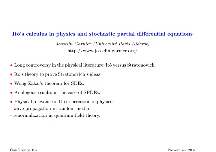
Itˆ o’s calculus in physics and stochastic partial differential equations Josselin Garnier (Universit´ e Paris Diderot) http://www.josselin-garnier.org/ • Long controversy in the physical literature: Itˆ o versus Stratonovich. • Itˆ o’s theory to prove Stratonovich’s ideas. • Wong-Zakai’s theorem for SDEs. • Analogous results in the case of SPDEs. • Physical relevance of Itˆ o’s correction in physics: - wave propagation in random media, - renormalization in quantum field theory. Conference Itˆ o November 2015

Itˆ o versus Stratonovich in SDEs • When white noise is approximated by a smooth process this often leads to Stratonovich interpretations of stochastic integrals, at least in one dimension. • Toy model: dX ε f ( X ε ) Y ε , = dt − 1 ε 2 Y ε dt + 1 dY ε = ε 2 dB. Y ε ( t ) looks like a white noise: Y ε Gaussian, E [ Y ε ( t )] = 0, and 2 ε 2 exp( − | t − t ′ | E [ Y ε ( t ) Y ε ( t ′ )] = ) → δ ( t − t ′ ), so the conjecture is: 1 ε 2 Y ε → dW dt and X ε → X (in dist.) with dX dt = f ( X ) dW dt . In fact, Itˆ o’s calculus shows that dX = f ( X ) dW + 1 2 f ′ ( X ) f ( X ) dt, which means dX = f ( X ) ◦ dW. Conference Itˆ o November 2015

Itˆ o versus Stratonovich in SDEs • Wong-Zakai: under fairly general circumstances, - if W ε denotes some “natural” smooth ε -approximation to a Brownian motion W , - if X ε denotes the solution to the ODE dX ε = h ( X ε ) + g ( X ε ) dW ε dt , dt then X ε → X (in dist.), the solution to the SDE dX = h ( X ) dt + g ( X ) ◦ dW, where ◦ dW denotes Stratonovich integration against W . It makes sense in the form dX = h ( X ) dt + g ( X ) dW + 1 2 g ′ ( X ) g ( X ) dt. ֒ → This result gives the right model for physical applications. Conference Itˆ o November 2015

Itˆ o versus Stratonovich in SDEs Beyond one-dimensional: • Toy model (Langevin equation): md 2 X ε f ( X ε ) Y ε − dX ε = dt , dt 2 − 1 ε 2 Y ε dt + 1 dY ε = ε 2 dB. The conjecture is: Y ε → dW dt and X ε → X with md 2 X dt 2 = f ( X ) dW dt − dX dt . Itˆ o’s calculus shows that this is correct: X ′ dt, dX = mdX ′ f ( X ) dW − X ′ dt. = Moreover X is smooth and the Itˆ o and Stratonovich integrals coincide. Conference Itˆ o November 2015

Itˆ o versus Stratonovich in SDEs Beyond one-dimensional: • Toy model: m 0 ε 2 d 2 X ε f ( X ε ) Y ε − dX ε = dt , dt 2 − 1 ε 2 Y ε dt + 1 dY ε = ε 2 dB. The conjecture is: Y ε → dW dt and X ε → X with dX dt = f ( X ) dW dt . In fact, Itˆ o’s calculus shows that 1 2(1 + m 0 ) f ′ ( X ) f ( X ) dt. dX = f ( X ) dW + The integral is nor Itˆ o (correction= 0) neither Stratonovich 2 f ′ ( X ) f ( X ) dt ). (correction= 1 Remark: If m 0 ε 2 → m 0 ε , then Itˆ o. If m 0 ε 2 → m 0 ε 3 , or m 0 ε 4 , or . . . , then Stratonovich. Conference Itˆ o November 2015

Itˆ o versus Stratonovich in SDEs Beyond one-dimensional: Smooth approximation to white noise in one dimension leads to the Stratonovich stochastic integral. This is not true in general, however, in the multidimensional case: an additional drift can appear in the limit. • Toy model: dX ε Y ε 1 = 1 , dt dX ε 2 Y ε = 2 , dt dX ε 3 ( X ε 1 Y ε 2 − X ε 2 Y ε = 1 ) , dt − 1 2 dt + 1 1 dt − α dY ε ε 2 Y ε ε 2 Y ε = ε 2 dB 1 , 1 − 1 1 dt + 1 2 dt + α dY ε ε 2 Y ε ε 2 Y ε = ε 2 dB 2 . 2 Conference Itˆ o November 2015

Itˆ o versus Stratonovich in SDEs We conjecture − 1         dW 1 dW 1 − α dW 2  Y ε  1 α 1 1  →  = dt dt dt     1 + α 2 Y ε dW 2 α dW 1 + dW 2 − α 1 2 dt dt dt and ( X ε 1 , X ε 2 , X ε 3 ) → ( X 1 , X 2 , X 3 ) with 1 dX 1 � dW 1 − αdW 2 � = , 1 + α 2 dt dt dt 1 dX 2 � dW 2 + αdW 1 � = , dt 1 + α 2 dt dt 1 dX 3 ( αX 1 − X 2 ) dW 1 + ( αX 2 + X 1 ) dW 2 � � = . 1 + α 2 dt dt dt Itˆ o and Stratonovich coincide. However the result is wrong! Correct answer: 1 α � � dX 3 = ( αX 1 − X 2 ) dW 1 + ( αX 2 − X 1 ) dW 2 + 1 + α 2 dt. 1 + α 2 The drift correction is related to the L´ evy area of the driving processes and the Lie brackets between the row vectors of the diffusion matrix. Conference Itˆ o November 2015

Itˆ o versus Stratonovich in SDEs In dimension d , with r approximations of Brownian motions W ε n [Ikeda and Watanabe, 1989]: r dX ε σ in ( X ε ) dW ε � + b i ( X ε ) i n = dt dt n =1 ↓ r r d σ in ( X ) dW n + b i ( X ) dt + 1 � � � � � dX i = c nm + s nm σ qn ( X ) ∂ x q σ im ( X ) dt 2 n =1 n,m =1 q =1 with the symmetric (Itˆ o-Stratonovich) correction c nm = δ nm and the antisymmetric (L´ evy) correction � � ε 2 dW ε dW ε 1 � W ε − W ε m n � � s nm = lim dt ε 2 E n m dt dt ε → 0 0 See also [Fouque et al, 2007] for weak convergence results. Conference Itˆ o November 2015

Itˆ o versus Stratonovich - Extension to SPDEs - part I • How to make sense of a stochastic PDE driven by noise dW dt white in time and colored in space of the type du = ∂ 2 x udt + H ( u ) dt + G ( u ) dW. We can use martingale theory and Itˆ o’s calculus for Hilbert-space valued processes to make sense of this equation. • Example: Itˆ o-Schr¨ odinger equation [Dawson and Papanicolaou, 1984]: idu = ∂ 2 x udt + u ◦ dW, where E [ W ( t, x ) W ( t ′ , x ′ )] = min( t, t ′ ) γ ( x − x ′ ). Conference Itˆ o November 2015

Itˆ o versus Stratonovich - Extension to SPDEs - part I • How to make sense of a stochastic PDE driven by noise dW dt white in time and colored in space of the type du = ∂ 2 x udt + H ( u ) dt + G ( u ) dW. We can use martingale theory and Itˆ o’s calculus for Hilbert-space valued processes to make sense of this equation. • Example: Itˆ o-Schr¨ odinger equation [Dawson and Papanicolaou, 1984]: x udt + udW − 1 idu = ∂ 2 2 γ (0) udt, where E [ W ( t, x ) W ( t ′ , x ′ )] = min( t, t ′ ) γ ( x − x ′ ). Conference Itˆ o November 2015

Wave propagation in random media ω 2 ∆ � x ˆ u ( � x ) + x ) ˆ u ( � x ) = f ( � x ) . c 2 ( � x = ( x , z ) ∈ R 2 × R . Denote � • Randomly layered medium model: 1 x ) = 1 � � 1 + µ ( z ) c 2 c 2 ( � 0 c 0 is a reference speed, µ ( z ) is a zero-mean random process. • Isotropic random medium model: 1 x ) = 1 � � 1 + µ ( � x ) c 2 c 2 ( � 0 c 0 is a reference speed, µ ( � x ) is a zero-mean random process. Conference Itˆ o November 2015

Wave propagation in the random paraxial regime • Consider the time-harmonic form of the scalar wave equation ( � x = ( x , z )) u + ω 2 ( ∂ 2 � � z + ∆ ⊥ )ˆ 1 + µ ( x , z ) u = δ ( z ) f ( x ) . ˆ c 2 0 Consider the paraxial regime: ω → ω ε 2 , z � x � x µ ( x , z ) → ε 3 µ � � f ( x ) → f ε 4 , , . ε 2 ε 2 φ ε (slowly-varying envelope of a plane wave) defined by The function ˆ ωz i ω, x ε 4 c 0 ˆ u ε ( ω, x , z ) = ε 4 e φ ε � � ˆ ε 2 , z satisfies φ ε + ω 2 � � 1 2 i ω x , z φ ε + φ ε + ∆ ⊥ ˆ z ˆ c 0 ∂ z ˆ � ˆ ε 4 ∂ 2 φ ε � = δ ( z ) f ( x ) . εµ c 2 ε 2 0 Conference Itˆ o November 2015

Wave propagation in the random paraxial regime • Consider the time-harmonic form of the scalar wave equation ( � x = ( x , z )) u + ω 2 ( ∂ 2 � � z + ∆ ⊥ )ˆ 1 + µ ( x , z ) u = δ ( z ) f ( x ) . ˆ c 2 0 Consider the paraxial regime: ω → ω ε 2 , z � x � x µ ( x , z ) → ε 3 µ � � f ( x ) → f ε 4 , , . ε 2 ε 2 φ ε (slowly-varying envelope of a plane wave) defined by The function ˆ i ωz ω, x ε 4 c 0 ˆ u ε ( ω, x , z ) = ε 4 e φ ε � � ˆ ε 2 , z satisfies φ ε + ω 2 � � 2 i ω 1 x , z φ ε + φ ε + ∆ ⊥ ˆ z ˆ c 0 ∂ z ˆ � ˆ ε 4 ∂ 2 φ ε � εµ = δ ( z ) f ( x ) . c 2 ε 2 0 • In the regime ε ≪ 1, the forward-scattering approximation in direction z is valid and φ ε satisfies the Itˆ φ = lim ε → 0 ˆ ˆ o-Schr¨ odinger equation [1] φ = ic 0 φdz + iω d ˆ 2 ω ∆ ⊥ ˆ ˆ φ ◦ dB ( x , z ) , 2 c 0 with B ( x , z ) Brownian field E [ B ( x , z ) B ( x ′ , z ′ )] = γ ( x − x ′ ) min( z, z ′ ), � ∞ −∞ E [ µ ( 0 , 0) µ ( x , z )] dz , and initial conditions: ˆ φ ( ω, x , z = 0) = ic 0 γ ( x ) = 2 ω f ( x ). [1] J. Garnier and K. Sølna, Ann. Appl. Probab. 19 , 318 (2009).