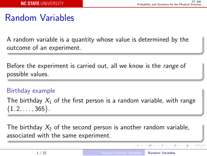
Random Variables A random variable is a quantity whose value is - PowerPoint PPT Presentation

ST 380 Probability and Statistics for the Physical Sciences Random Variables A random variable is a quantity whose value is determined by the outcome of an experiment. Before the experiment is carried out, all we know is the range of possible values. Birthday example The birthday X 1 of the first person is a random variable, with range { 1 , 2 , . . . , 365 } . The birthday X 2 of the second person is another random variable, associated with the same experiment. 1 / 22 Discrete Random Variables Random Variables

ST 380 Probability and Statistics for the Physical Sciences Birthday example The quantity X defined by � 0 if no two people have the same birthday X = 1 otherwise is a random variable, and X = 1 if and only if A occurs. Bernoulli Random Variable Any random variable whose only possible values are 0 and 1 is called a Bernoulli random variable . 2 / 22 Discrete Random Variables Random Variables

ST 380 Probability and Statistics for the Physical Sciences Example 3.4 9-volt batteries are tested until one with an acceptable voltage is obtained. The sample space is S = { A , UA , UUA , . . . } . Define X by X = number of batteries tested . Then X ( A ) = 1 X ( UA ) = 2 X ( UUA ) = 3 . . . The range of X is { 1 , 2 , 3 , . . . } , a countably infinite set. 3 / 22 Discrete Random Variables Random Variables

ST 380 Probability and Statistics for the Physical Sciences Example 3.5 Y is the altitude at a randomly chosen location in the U.S. The range of Y is the real number interval [ − 282 , 14494], an uncountably infinite set. 4 / 22 Discrete Random Variables Random Variables

ST 380 Probability and Statistics for the Physical Sciences Discrete and Continuous Random Variables Discrete Random Variable: A random variable whose range is finite or countably infinite. Continuous Random Variable: A random variable Y satisfying: its range is the union of one or more real number intervals; 1 P ( Y = c ) = 0 for every c in the range of Y . 2 Note For a continuous random variable Y , P ( c − ǫ ≤ Y ≤ c + ǫ ) could be positive for any ǫ > 0, but decreases to 0 as ǫ becomes smaller. 5 / 22 Discrete Random Variables Random Variables

ST 380 Probability and Statistics for the Physical Sciences Probability Distributions for Discrete Random Variables To calculate the probability of any event defined by a discrete random variable X , we need a list of the possible values (the range ) of X , and the probability of each. Probability Mass Function The probability mass function (pmf) p of a discrete random variable X is p ( x ) = P ( X = x ) = P ( { s ∈ S : X ( s ) = x } ) for any x in the range of X . 6 / 22 Discrete Random Variables Discrete Probability Distributions

ST 380 Probability and Statistics for the Physical Sciences Every pmf must satisfy: p ( x ) ≥ 0 for all x in the range of X and � p ( x ) = 1 . x ∈ range of X Any function p with these properties could be the pmf of some discrete random variable. 7 / 22 Discrete Random Variables Discrete Probability Distributions

ST 380 Probability and Statistics for the Physical Sciences Parameter of a Distribution Recall that a Bernoulli random variable X is one that takes only the values 0 and 1. Suppose that P ( X = 1) = α , for some α between 0 and 1; then the pmf of X is: � x = 1 α p ( x ) = 1 − α x = 0 . This is a different pmf for different α ; we write it as p ( x ; α ), and call it a family of distributions (or pmfs), indexed by the parameter α . 8 / 22 Discrete Random Variables Discrete Probability Distributions

ST 380 Probability and Statistics for the Physical Sciences Geometric Distribution Recall Example 3.4: 9-volt batteries are tested until one with an acceptable voltage is obtained. The sample space is S = { A , UA , UUA , . . . } . Define X by X = number of batteries tested . Then X ( A ) = 1 X ( UA ) = 2 X ( UUA ) = 3 . . . 9 / 22 Discrete Random Variables Discrete Probability Distributions

ST 380 Probability and Statistics for the Physical Sciences So p (1) = P ( X = 1) = P ( A ) = p p (2) = P ( X = 2) = P ( UA ) = P ( U ) P ( A ) = (1 − p ) p p (3) = P ( X = 3) = P ( UUA ) = P ( U ) P ( U ) P ( A ) = (1 − p ) 2 p . . . In general, p ( x ) = p ( x ; p ) = p (1 − p ) x − 1 , x = 1 , 2 , . . . This is the geometric family of distributions, with parameter p . 10 / 22 Discrete Random Variables Discrete Probability Distributions

ST 380 Probability and Statistics for the Physical Sciences Looking Ahead In many problems we observe a random variable X , and we may know that its distribution belongs to a particular parametric family. But we typically do not know the value of the parameter; a central problem in statistics is making inferences about the values of parameters: parameter estimation , etc. 11 / 22 Discrete Random Variables Discrete Probability Distributions

ST 380 Probability and Statistics for the Physical Sciences Cumulative Distribution Function For a given random variable X , we often need the probability P ( X ≤ x ) for some real number x . It is convenient to define it as a function, the cumulative distribution function (cdf) F ( x ) = P ( X ≤ x ) , −∞ < x < ∞ . If X is discrete, we can construct F ( x ) from the pmf p ( x ): � F ( x ) = p ( y ) . y in the range of X with y ≤ x 12 / 22 Discrete Random Variables Discrete Probability Distributions

ST 380 Probability and Statistics for the Physical Sciences The graph of F ( x ) against x is constant between values of X , with jump of size P ( X = x ) = p ( x ) at each possible value of X . So from the locations of the jumps in F ( x ) we can identify the range of X , and from the sizes of the jumps we can identify its pmf. That is, the pmf and cdf carry the same information. Either can be derived from the other, and each provides a complete description of the probability distribution of X . 13 / 22 Discrete Random Variables Discrete Probability Distributions

ST 380 Probability and Statistics for the Physical Sciences Expected Values The Expected Value of X Let X be a discrete random variable with range D and pmf p ( x ) , x ∈ D . The expected value of X is � E ( X ) = xp ( x ) . x ∈ D The expected value is sometimes written µ X , and sometimes called the mean value. Expected value is just a weighted average of the values of X , weighted by their probabilities. 14 / 22 Discrete Random Variables Expected Values

ST 380 Probability and Statistics for the Physical Sciences Interpreting Expected Value Recall the interpretation of probability as the relative frequency in a large number n of trials. For each possible value x of X , let n ( x ) be the number of times that X takes the value x . Then the sum of the observed values of X is � xn ( x ) , x ∈ D and their average is � x ∈ D xn ( x ) x n ( x ) � = n . n x ∈ D 15 / 22 Discrete Random Variables Expected Values

ST 380 Probability and Statistics for the Physical Sciences But when n is large, we expect n ( x ) ≈ p ( x ) , n so x n ( x ) � � ≈ xp ( x ) = E ( X ) n x ∈ D x ∈ D That is, we expect the sample average in many trials to be close to the expected value . 16 / 22 Discrete Random Variables Expected Values

ST 380 Probability and Statistics for the Physical Sciences Bernoulli Family If X has the Bernoulli distribution with parameter α , then D = { 0 , 1 } , and E ( X ) = 0 × P ( X = 0) + 1 × P ( X = 1) = α. Geometric Family If X has the geometric distribution with parameter p , then D = { 1 , 2 , . . . } , and ∞ ∞ xp (1 − p ) x − 1 = 1 � � E ( X ) = xP ( X = x ) = p . x =1 x =1 Note that when D is infinite, the series defining E ( X ) may converge to infinity, or not converge at all. 17 / 22 Discrete Random Variables Expected Values

ST 380 Probability and Statistics for the Physical Sciences Expected Value of a Function of X If X is a random variable, and h ( x ) is some function (such as h ( x ) = x 2 or h ( x ) = cos(2 π x )), then Y = h ( X ) is also a random variable. Not surprisingly, � E ( Y ) = E [ h ( X )] = h ( x ) p ( x ) . x ∈ D 18 / 22 Discrete Random Variables Expected Values

ST 380 Probability and Statistics for the Physical Sciences Rules of Expected Value In the special case where h ( x ) is a linear function, say h ( x ) = ax + b , we find E [ h ( X )] = E ( aX + b ) � = ( ax + b ) p ( x ) x ∈ D � � � � � � = xp ( x ) + p ( x ) a b x ∈ D x ∈ D = aE ( X ) + b . 19 / 22 Discrete Random Variables Expected Values

ST 380 Probability and Statistics for the Physical Sciences Variance If the random variable X has expected value µ , then its variance is V ( X ) = E [( X − µ ) 2 ] . Standard Deviation The variance of X is sometimes written σ 2 X , and its standard deviation is � σ X = V ( X ) . Standard deviation is in the same units as X , and represents (in a root-mean-square sense) how far you can expect X to differ from µ . 20 / 22 Discrete Random Variables Expected Values

ST 380 Probability and Statistics for the Physical Sciences Shortcut Formula for Variance V ( X ) = E [( X − µ ) 2 ] = E ( X 2 − 2 µ X + µ 2 ) = E ( X 2 ) − 2 µ E ( X ) + µ 2 = E ( X 2 ) − µ 2 . Bernoulli Family If X has the Bernoulli distribution with parameter α , then µ = α , and X 2 = X , so V ( X ) = α − α 2 = α (1 − α ) . 21 / 22 Discrete Random Variables Expected Values