Lecture 9 : Change of discrete random variable 0/ 13 You have - PowerPoint PPT Presentation

Lecture 9 : Change of discrete random variable 0/ 13

You have already seen (I hope) that whenever you have “variables” you need to consider change of variables . Random variables are no different. The notion of “change of random variable” is handled too briefly on page 112 and 115 (the meaning of the symbol h ( X ) is not even defined in the text). This is something I will test you on. Example 1 � � 3 , 1 Suppose X ∼ Bin . 2 line graph 1 2 3 0 table x 0 1 2 3 1 3 3 1 (b) P ( X = x ) 8 8 8 8 1/ 13 Lecture 9 : Change of discrete random variable

Suppose we want to define a new random variable Y = 2 X − 1. How do we do it? So how do we define P ( Y = k ) ? Answer - express Y in terms of X and compute so P ( Y = k ) = P ( 2 X − 1 = k ) � X = k + 1 � = P (*) 2 The right-hand site is the logical definition of the left-hand side. But as is often the case in probability it is easier to pretend we know what P ( Y = k ) means already and then the last two steps are a computation. 2/ 13 Lecture 9 : Change of discrete random variable

So let’s compute the pmf of Y . What are the possible values of Y ? From (*) k is a possible value of Y ⇔ k + 1 is a possible values of X . 2   0 − 1       ⇐⇒ k + 1  1  1     = Y =   ⇐⇒ 2 3 2            3  5   Note possible value possible value of of 3/ 13 Lecture 9 : Change of discrete random variable

So the possible values of Y are obtained by applying the function h ( x ) = 2 x − 1 to the possible values of X . (note Y = f ( X ) ). 0 1 1 3 2 5 3 possible values possible values of of Just “push forward” the values of X. 4/ 13 Lecture 9 : Change of discrete random variable

Now we have computed the possible values of Y we need to compute their probabilities. Just repeat what we did P ( Y = − 1 ) = P ( 2 X − 1 = − 1 ) = P ( X = 0 ) = 1 8 P ( Y = 1 ) = P ( 2 X − 1 = 1 ) = P ( X = 1 ) = 3 8 Similarly P ( Y = 3 ) = 3 P ( Y = 5 ) = 1 and 8 8 y − 1 1 3 5 1 3 3 1 P ( Y = y ) 8 8 8 8 5/ 13 Lecture 9 : Change of discrete random variable

So we have the “same probabilities” as before namely 1 8, 3 8, 3 8, 1 8 it is just then are pushed-forward to new locations 0 1 2 1 3 5 3 6/ 13 Lecture 9 : Change of discrete random variable

Example 2 (Probabilities can “coalesce”) There is one tricky point. Several different possible values of X can push-forward to the same values of Y . We now give an example. Suppose X has pmf 0 1 That is P ( X = − 1 ) = 1 P ( X = 0 ) = 1 P ( X = 1 ) = 1 4 , 2 , 4 We will make the change of variable Y = X 2 . So what happens when we push forward the three values − 1, 0, 1 by h ( x ) = x 2 . We get only the two values 0 and 1. h ( x ) − 1 1 − − − → 0 0 − − − → 1 1 − − − → 7/ 13 Lecture 9 : Change of discrete random variable

What happens with the corresponding probabilities P ( Y = 0 ) = P ( X 2 = 0 ) = P ( X = 0 ) = 1 2 But P ( Y = 1 ) = P ( X 2 = 1 ) = P ( X = 1 or X = − 1 ) = P (( X = 1 ) ∪ ( X − 1 )) = P ( X = 1 ) + P ( X = − 1 ) = 1 4 + 1 4 = 1 2 8/ 13 Lecture 9 : Change of discrete random variable

So we set 0 1 y 1 1 P ( Y = y ) 2 2 So, 0 1 0 1 Think of two masses (probabilities) of mass 1 4, one at − 1, and one at ! coalescing into a combined mass of 1 2 at 0. 9/ 13 Lecture 9 : Change of discrete random variable

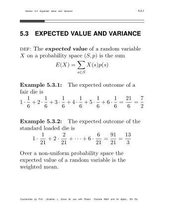
The Expected Value Formula If h ( x ) in the transformation law Y = h ( X ) is complicated it can be very hard to explicitly compute the pmf of Y . Amazingly we can compute the expected value E ( Y ) using the old proof p X ( x ) of X according to Theorem 3 � � E ( h ( X )) = h ( x ) p X ( x ) = h ( x ) P ( X = x ) possible possible values values of X of X 10/ 13 Lecture 9 : Change of discrete random variable

We will illustrate this with the pmf ’s of Example 1. First we compute E ( Y ) using the definition of E ( Y ) . y − 1 1 3 5 ( ♯ ) 1 3 3 1 P ( Y = y ) 8 8 8 8 � E ( Y ) = y P ( Y = y ) possible value of Y � 1 � � 3 � � 3 � � 1 � = ( − 1 ) + ( 1 ) + ( 3 ) + ( 5 ) 8 8 8 8 = − 1 + 3 + 9 + 5 8 = 16 8 = 2 11/ 13 Lecture 9 : Change of discrete random variable

Notice to do the previous computations we needed the table ( ♯ ) which we computed five pages ago. Now we use the Theorem . So now we use that Y is a function of the random variable X and use the proof of X from the table on page 1. x 0 1 2 3 (b) 1 3 3 1 P ( X = x ) 8 8 8 8 � E ( X ) = h ( x ) P ( X = x ) possible values of X � = ( 2 x − 1 ) P ( X = x ) x = 0 , 1 , 2 , 3 � 1 � � 3 � � 5 � � 3 � = ( − 1 ) + ( 1 ) + ( 3 ) + ( 5 ) = 2 8 8 8 8 12/ 13 Lecture 9 : Change of discrete random variable

The most common change of variable is linear Y = aX + b so we will give formulas to show how expected value and variance behave under such a change. Theorem (i) E ( aX + b ) = aE ( X ) + b (ii) V ( aX + b ) = a 2 V ( X ) (so V ( − X ) = V ( X ) ) 13/ 13 Lecture 9 : Change of discrete random variable