R Programming Basics Thomas J. Leeper May 20, 2015 1 Functions - - PDF document

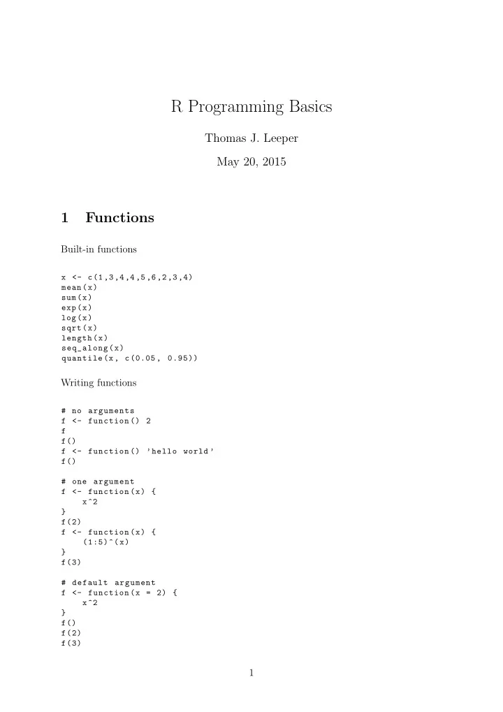
R Programming Basics

Thomas J. Leeper May 20, 2015

1 Functions

Built-in functions

x <- c(1,3,4,4,5,6,2,3,4) mean(x) sum(x) exp(x) log(x) sqrt(x) length(x) seq_along(x) quantile(x, c(0.05 , 0.95))

Writing functions

# no arguments f <- function () 2 f f() f <- function () ’hello world ’ f() # one argument f <- function(x) { x^2 } f(2) f <- function(x) { (1:5)^(x) } f(3) # default argument f <- function(x = 2) { x^2 } f() f(2) f(3)

1

# multiple arguments f <- function(x, y) { x - y } # mutliple arguments , some defaults f <- function(x, y = 2) { x - y } # return values f <- function(x) { y <- combn(x, 2) min(colSums(y)) } # list return values f <- function(x) { list(mean = mean(x), range = range(x), sd = sd(x)) } f(1:6) f(1:6) $mean # etc.

Some things to remember about functions:

• Argument recycling. Remember that vectorized operations almost always involve

recycling, even if you don’t expect it:

f <- function(x, y) { x + y } f(1:6, 2) f(1:6, 1:2)

• Environments: A confusing aspect of functions is the notion of an evaluation envi-
• ronment. Inside a function, variables take on values as specified by the function’s
• arguments. If no value is specified for an argument and the argument has no default

value, the function will fail to work:

f <- function(x) x^2 f()

• Variable scope: A more complicated issue relates to how variables that are not

function arguments are handled inside functions: 2

z <- 1 f <- function(x) { x + z } f() f(1)

In the above example, z is taken from the function’s parent environment. This can create confusion because a function can both retrieve variables from its parent environment and modify the values of those variables. Both of these lack referential transparency because calling a function on an object can result in the original

• bject being modified. Stata actually works entirely on violating the notion of the

referential transparency, so this is an important distinction between how R and Stata behave.1

• Generic functions and method dispatch: R implements a system of functional pro-

gramming that involves “generic” functions and class-specific methods. This means that the same function (e.g., print or summary) can be used to produce different results for objects of different classes. A classic example of this is summary, which produces radically different output for different kinds of objects:

summary(mtcars) summary(mtcars$cyl) summary(lm(mpg ~ cyl , data = mtcars ))

• Lazy evaluation: This is not important for your assignment but it might be some-

thing you encounter. Arguments to functions are evaluated lazily, which means that they are not evaluated until they are actually requested by a function, which means they may do things you find unintuitive:

x <- 1 z <- 1 f <- function(x, z = x^2) z f(x = 2) # what do you expect this to be? f(z = 2) # what do you expect this to be?

Questions?

1You can violate referential transparency in R, and there is in principle nothing wrong with that but

it can create confusion if you are unprepared for it.

3

2 Repeated Operations

In order to do many computation tasks, we need to be able to repeat an R expression multiple times or evaluate a function over a range of values. We can write vectorized functions to do some of this, but not always. The following are some strategies for repeating code.

• Looping: for

for(i in c(1 ,2 ,3)) { print(i) } x <- numeric (3) for(i in seq_along(x)) { x <- i * 2 }

• Looping: while

x <- TRUE i <- 0 while(x) { i <- i + 1 print(i) if(i == 10) break }

• The apply and *apply-family functions

mean (1:5) # vectorized lapply (1:5, mean) sapply (1:5, mean) m <- matrix (1:16 , nrow = 4) apply(m, 1, sum) apply(m, 2, sum) # Use ‘mapply ‘ f <- function(x, y) { x + y } mapply(f, x = 1:3, y = 1:3)

• Using replicate to repeat an expression

4

rnorm (1) + rnorm (1) replicate (5, rnorm (1) + rnorm (1))

Questions?

3 Simulation Methods

Simulation methods allow us to solve lots of problems when we either (1) cannot find a closed form mathematical solution to a statistical problem and/or (2) when we think it is inappropriate to rely on a particular parametric assumption (e.g., that a statistic is normally distributed). Simulation methods involve sampling and/or random number generation in tandem with repeated evaluation of a function or expression.

• Generating random numbers and using sample

# pseudo -RNG rnorm (1) rnorm (5) rnorm(5, mean = 3, sd = 2) rpois(5, 3) # set RNG seed set.seed (1) rnorm (5) set.seed (1) rnorm (5) # sample sample (2:6, 1) sample (2:6, 5) sample (2:6, 10, TRUE)

• Simple repeated sampling

set.seed (1) x <- rnorm (1e6 , 5, 1) mean(x) s1 <- sample(x, 10, FALSE) mean(s1) s2 <- sample(x, 1e3 , FALSE) mean(s2) r1 <- replicate (1000 , mean(sample(x, 10, FALSE ))) r2 <- replicate (1000 , mean(sample(x, 1e3 , FALSE )))

5

mean(r1) mean(r2) sd(r1) sd(r2)

• The Bootstrap. This is useful for estimating variance/SD/SE for estimators that

do not have a closed form variance calculation, and in many other contexts (e.g., non-independent observations, etc.). Let’s look at a simple example: median.

set.seed (1) x1 <- rnorm (1e6 , 5, 1) mean(x1) median(x1) s <- sample(x1 , 1e3 , FALSE) mean(s) median(s) b <- replicate (1000 , mean(sample(s, 1e3 , TRUE ))) mean(b) # mean of bootstrapped means sd(b) # sd of bootstrapped means quantile(b, c(0.025 ,0.975)) # 95 % CI for mean b <- replicate (1000 , median(sample(s, 1e3 , TRUE ))) mean(b) # mean of bootstrapped medians sd(b) # sd of bootstrapped medians quantile(b, c(0.025 ,0.975)) # 95 % CI for median

• Bootstrapping OLS

# function to estimate model one time

• nce <- function(X, y) {

b <- solve(t(X) %*% X) %*% t(X) %*% y } # bootstrap n <- 5000 bootmat <- matrix(numeric (), ncol = 3, nrow = n) for(i in 1:n) { s <- sample (1: nrow(X), nrow(X), TRUE) Xtmp <- X[s,] ytmp <- y[s] tried <- try(once(Xtmp , ytmp )) if(! inherits(tried , ’try -error ’)) bootmat[i,] <- tried } # bootstrapped coefficient estimates apply(bootmat , 2, mean , na.rm = TRUE) # bootstrapped standard errors

6

apply(bootmat , 2, sd , na.rm = TRUE) # jackknife jackmat <- matrix(numeric (), ncol = 3, nrow = nrow(X)) for(i in 1: nrow(X)) { Xtmp <- X[-i,] ytmp <- y[-i] tried <- try(once(Xtmp , ytmp )) if(! inherits(tried , ’try -error ’)) jackmat[i,] <- tried } # bootstrapped coefficient estimates apply(jackmat , 2, mean , na.rm = TRUE) # bootstrapped standard errors apply(jackmat , 2, sd , na.rm = TRUE)

• Jackknife

set.seed (1) x1 <- rnorm (1e6 , 5, 1) s <- sample(x1 , 1e3 , FALSE) mean(s) j <- numeric(length(s)) for(i in seq_along(s)) j[i] <- mean(s[-i]) mean(s) sd(s) quantile(s, c(0.025 , 0.975))

Questions?

4 Optimization

Recall the objective of maximum likelihood estimation. We have some data which rep- resent a sample from a population. The population distribution is governed by some parameters, θ, and we want to use our sample data to estimate (or infer) the values of those parameters. MLE is the process of finding the values of θ that make our sample data most likely. In other words, given θ takes some set of values, how likely are we to

• bserve the data we actually saw? If θ had some other set of values, how likely would we

be to observe our data? etc. etc. The Likelihood function is a statement of this conditional probability: L(θ|data). We want to “maximize” this function. When the maximum is highest, we have found the input parameter values for θ that make our data most likely. This in turn tells us that 7

these are the parameters most likely to have generated our sample data, and thus the population data from which the sample data are drawn. L is just a product of the likelihoods of observing each case in our data, so: L(θ|X) = L1 + L2 + . . . =

n

• i=1

Li = p(x1|θ) + p(x2|θ) + . . . =

n

• i=1

p(x1|θ) It is often more convenient to work with log likelihoods: ln L = n

i=1 ln p(xi|θ). This

transformation is possible because of the property: log(x ∗ y) = log(x) + log(y). Why do we do this? Simplicity but also floating-point issues (because small numbers multiplied by each other go to zero, our likelihood can end up beyond the precision of contemporary computers). Stating our likelihood function requires making a parametric assumption (i.e., we have to choose a family of probability distributions defined by parameters θ that will indicating how likely a given observation is). Once we’ve defined our likelihood function, we simply evaluate that function (with dif- ferent possible values for θ) at the observed values of our data and select the values θ yielding the highest (log-)likelihood. Likelihood function for a simple example involving a proportion of heads coin tosses. We want to find the parameter π that makes this set of heads most likely: L(π|heads) = Pr(heads|π) = πheads(1 − π)tails Here’s the corresponding Log likelihood function: ln L(π) = heads ln(π) + tails ln(1 − π) 8

Here’s how we represent that in R (note how π is written as x):

ll <- function(x, heads = 7, n = 10) { heads*log(x) + (n-heads )*log(1-x) }

How do we find the maximum likelihood estimate? We can do this in three ways:

• Analytical
• Grid search
• Optimization

Analytical is only available for some problems. Grid search is slow. Optimization is fastest and most general. Analytic solution involves taking the derivative of the log likelihood, which is called the score function: d ln L(π) dπ = heads π + tails 1 1 − π(−1) = heads π − tails 1 − π Solve for parameter π to find the maximum likelihood estimate: d ln L(π) dπ = heads π − tails 1 − π 0 = heads π − tails 1 − π tails 1 − π = heads π π(tails) = (1 − π)heads π(n − x) = (1 − π)(x) nπ − xπ = x − xπ nπ = x π = x n 9

That provides a simple analytic solution. To perform a grid search, we simply specify a set of possible values of our parameter, calculate the likelihood for each and pick the one that is largest.

possible <- seq(0,1, by = 0.05)

• ut <- sapply(possible , ll)
• ut

which.max(out) possible[which.max(out)] # plot of log -likelihood curve(ll , from = 0, to = 1) points(possible , out , col = ’blue ’, pch = 18) points(possible[which.max(out)], out[which.max(out)], col = ’red ’, pch = 15) abline(v = possible[which.max(out)], col = ’red ’) # override defaults

• ut <- sapply(possible , ll , heads = 4, n = 10)

In R, ‘optim‘ is a minimization tool, so we always need to negate our function unless we set ‘control‘.

# function to minimize negll <- function(x, heads , n) {

• (heads*log(x) + (n-heads )*log(1-x))

} # minimize using ‘negll ‘

• ptim(p = 0.5, negll , heads = 7, n = 10, lower = 0, upper = 1, method = ’Brent ’)

# maximize using ‘ll ‘

• ptim(p = 0.5, ll , heads = 7, n = 10, lower = 0, upper = 1,

method = ’Brent ’, control = list(fnscale =

• 1))

Now let’s do a more complex problem, such as the coefficients for a Probit regression

• model. Let’s do something trivial like predict whether a car is automatic as a function
• f its horsepower:

m <- glm(am ~ hp , data = mtcars , family = binomial(link = "probit ")) summary(m)

How do we obtain the MLE of this model? We have to start by writing out a likelihood function, then maximize that function. The likelihood function will take possible param- eter values (i.e., coefficients) as inputs and evaluate our sample data given those possible coefficient values. In other words, if the intercept and slope were actually θ, what is the probability of seeing the values of y that we actually observe in our data: 10

L(β) =

n

• i=1

(πi)yi(1 − πi)(1 − yi) ln L(β) =

n

• i=1

ln((πi)yi(1 − πi)1−yi) =

n

• i=1

yi ln(πi) + (1 − yi) ln(1 − πi) =

n

• i=1

yi ln(φ(Xiβ)) + (1 − yi) ln(1 − φ(Xiβ)) The last step given πi = φ(Xiβ) (the inverse link function for the probit model). For the logit model, this inverse-link function is pii = eXiβ 1 + eXiβ . Here’s how we represent that in R:

ll <- function(beta , X, y) { p <- pnorm(X %*% beta) lik <- y * log(p) + (1-y) * log(1-p) sum(lik) }

Now we can solve this using a grid search:

X <- cbind (1, mtcars$hp) y <- mtcars$am iseq <- seq(-5, 5, by = 0.05) sseq <- seq (-0.08, 0.08, by = 0.005) g <- expand.grid(intercept = iseq , slope = sseq) grid_search <- apply(g, 1, function(z) ll(beta = z, X = X, y = y)) # estimated parameter values g[which.max(grid_search), ] # 3-D plot of log -likelihood function tmp <- grid_search tmp[tmp == -Inf] <- -1e3 persp(x = iseq , y = sseq , z = matrix(tmp , nrow = length(iseq)), xlim = c(-5, 5), ylim = c(-0.1, 0.1), zlim = c(-1e3 , 0), theta = 45, phi = 20, shade = 0.25, col = ’lightblue ’, border = NA) # heatmap of log -likelihood function image(x = iseq , y = sseq , z = matrix(tmp , nrow = length(iseq)), col = rainbow (1e4 , start = 0.1, end = 1))

Or using optim: 11

• pt <- optim(par = c(0,0), ll , X = X, y = y,

control = list(fnscale =

• 1), hessian = TRUE , method = "BFGS ")

The reason we ask for hessian = TRUE is this is what provides us standard errors:

• pt$hessian

sqrt(diag(solve(-opt$hessian ))) # compare to original results

• pt

sqrt(diag(solve(-opt$hessian ))) summary(m)

Questions? 12