Probability Theory Defd in terms of a probability space or sample - PowerPoint PPT Presentation

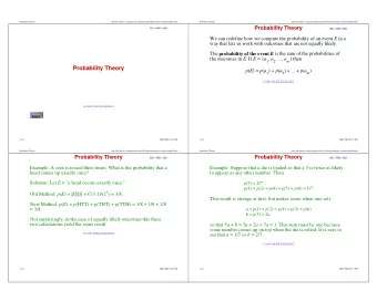
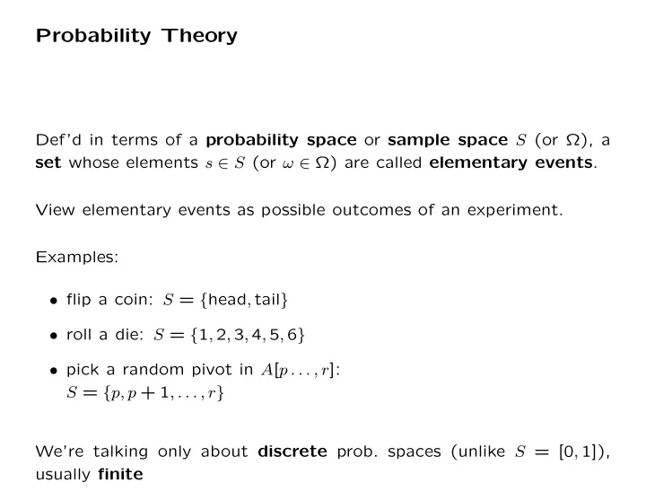
Probability Theory Def’d in terms of a probability space or sample space S (or Ω ), a set whose elements s ∈ S (or ω ∈ Ω) are called elementary events . View elementary events as possible outcomes of an experiment. Examples: • flip a coin: S = { head , tail } • roll a die: S = { 1 , 2 , 3 , 4 , 5 , 6 } • pick a random pivot in A [ p . . . , r ] : S = { p, p + 1 , . . . , r } We’re talking only about discrete prob. spaces (unlike S = [0 , 1] ), usually finite

An event is a subset of the prob. space Examples: • roll a die; A = { 2 , 4 , 6 } ⊂ { 1 , 2 , 3 , 4 , 5 , 6 } is the event of having an even outcome • flip two distinguishable coins: S = { HH, HT, TH, TT } , and A = { TT, HH } ⊂ S is the event of having the same outcome with both coins We say S (the entire sample space) is a certain event , and ∅ (the empty event) is a null event We say events A and B are mutually exclusive if A ∩ B = ∅

Axioms A probability distribution P () on S is mapping from events of S to reals s.t. 1. P ( A ) ≥ 0 for all A ⊆ S 2. P ( S ) = 1 (normalisation) 3. P ( A ) + P ( B ) = P ( A ∪ B ) for any two mutually exclusive events A and B , i.e., with A ∩ B = ∅ . Generalisation: for any finite sequence of pairwise mutually exclu- sive events A 1 , A 2 , . . .    = � � P A i P ( A i ) i i P ( A ) is called probability of event A

A bunch of stuff that follows: 1. P ( ∅ ) = 0 2. If A ⊆ B then P ( A ) ≤ P ( B ) 3. With ¯ A = S − A , we have P ( ¯ A ) = P ( S ) − P ( A ) = 1 − P ( A ) 4. For any A and B ( not necessarily mutually exclusive), P ( A ∪ B ) = P ( A ) + P ( B ) − P ( A ∩ B ) ≤ P ( A ) + P ( B ) Considering discrete sample spaces, we have for any event A � P ( A ) = P ( s ) s ∈ A If S is finite, and P ( s ∈ S ) = 1 / | S | , then we have uniform probability distribution on S (that’s what’s usually referred to as “picking an element of S at random”)

Conditional probabilities When you already have partial knowledge Example: a friend rolls two fair dice (prob. space is { ( x, y ) : x, y ∈ { 1 , . . . , 6 }} ) tells you that one of them shows a 6 . What’s the proba- bility for a 6 − 6 outcome? Information eliminates outcomes without any 6 , i.e., all combinations of 1 through 5 . There are 5 2 = 25 of them. The original prob. space has size 6 2 = 36 , thus we’re left with 36 − 25 = 11 events where at least one 6 is involved. These are equally likely, thus the sought probability must be 1 / 11 . The conditional probability of event A given that another event B occurs is P ( A | B ) = P ( A ∩ B ) P ( B ) given P ( B ) � = 0

In example: { (6 , 6) } A = { (6 , x ) : x ∈ { 1 , . . . , 6 }} ∪ B = { ( x, 6) : x ∈ { 1 , . . . , 6 }} with | B | = 11 (the (6 , 6) is in both parts) and thus P ( A ∩ B ) = P ( { (6 , 6) } ) = 1 / 36 and P ( A | B ) = P ( A ∩ B ) = 1 / 36 11 / 36 = 1 P ( B ) 11

Independence We say two events are independent if P ( A ∩ B ) = P ( A ) · P ( B ) equivalent to (if P ( B ) � = 0 ) to = P ( A ∩ B ) = P ( A ) · P ( B ) def P ( A | B ) = P ( A ) P ( B ) P ( B ) Events A 1 , A 2 , . . . , A n are pairwise independent if P ( A i ∩ A j ) = P ( A i ) · P ( A j ) for all 1 ≤ i < j ≤ n . They are (mutually) independent if every k -subset A i 1 , . . . , A i k , 2 ≤ k ≤ n and 1 ≤ i 1 < i 2 < · · · < i k ≤ n satisfies P ( A i 1 ∩ · · · ∩ A i k ) = P ( A i 1 ) · · · P ( A i k )

Random variables Reminder: we’re talking discrete probability spaces (makes things easier) A random variable (r.v.) X is a function from a probability space S to the reals, i.e., it assigns some value to elementary events Event “ X = x ” is def’d to be { s ∈ S : X ( s ) = x } Example: roll three dice • S = { s = ( s 1 , s 2 , s 3 ) | s 1 , s 2 , s 3 ∈ { 1 , 2 , . . . , 6 }} | S | = 6 3 = 216 possible outcomes • Uniform distribution: each element has prob 1 / | S | = 1 / 216 • Let r.v. X be sum of dice, i.e., X ( s ) = X ( s 1 , s 2 , s 3 ) = s 1 + s 2 + s 3

P ( X = 7) = 15 / 216 because 115 214 313 412 511 124 223 322 421 133 232 331 142 241 151 Important: With r.v. X , writing P ( X ) does not make any sense; P ( X = something ) does , though (because it’s an event ) Clearly, P ( X = x ) ≥ 0 and � x P ( X = x ) = 1 (from probability axioms) If X and Y are r.v. then P ( X = x and Y = y ) is called joint prob. dis- tribution of X and Y . � P ( Y = y ) = P ( X = x and Y = y ) x � P ( X = x ) = P ( X = x and Y = y ) y

R.v. X, Y are independent if ∀ x, y , events “ X = x ” and “ Y = y ” are independent Recall: A and B are independent iff P ( A ∩ B ) = P ( A ) · P ( B ) . Now: X, Y are independent iff ∀ x, y , P ( X = x and Y = y ) = P ( X = x ) · P ( Y = y ) Intuition: “ X = x ′′ = “ X = x and Y =? ′′ A = “ Y = y ′′ = “ X =? and Y = y ′′ = B “ X = x and Y = y ′′ A ∩ B =

Welcome to. . . expected values of r.v. Also called expectations or means Given r.v. X , its expected value is � E [ X ] = x · P ( X ) x Well-defined if sum is finite or converges absolutely Sometimes written µ X (or µ if context is clear) Example: roll a fair six-sided die, let X denote expected outcome E [ X ] = 1 · 1 / 6 + 2 · 1 / 6 + 4 · 1 / 6 + 5 · 1 / 6 + 6 · 1 / 6 = 1 / 6 · (1 + 2 + 3 + 4 + 5 + 6) = 1 / 6 · 21 = 3 . 5

Another example: flip three fair coins For each head you win $4, for each tail you lose $3 Let r.v. X denote your win. Then the probability space is { HHH,HHT,HTH,THH,HTT,THT,TTH,TTT } and E [ X ] = 12 · P ( 3H ) + 5 · P ( 2H ) − − 2 · P ( 1H ) − 9 · P ( 0H ) = 12 · 1 / 8 + 5 · 3 / 8 − 2 · 3 / 8 − 9 · 1 / 8 12 + 15 − 6 − 9 = 12 = 8 = 1 . 5 8 which is intuitively clear: each single coin contributes an expected win of 0 . 5 Important: Linearity of expectations E [ X + Y ] = E [ X ] + E [ Y ] whenever E [ X ] and E [ Y ] are defined True even if X and Y are not independent

Some more properties Given r.v. X and Y with expectations, constant a • E [ aX ] = aE [ X ] (note: aX is a r.v.) • E [ aX + Y ] = E [ aX ] + E [ Y ] = aE [ X ] + E [ Y ] • if X, Y independent , then � � E [ XY ] = xyP ( X = x and Y = y ) x y � � = xyP ( X = x ) P ( Y = y ) x y �   �� � = xP ( X = x ) yP ( Y = y )  x y = E [ X ] E [ Y ]

Variance The expected value of a random variable does not tell how “spread out” the variables are. Example: Two variables X and Y . P(X=1/4)=P(X=3/4)=1/2 P(Y=0)=P(Y=1)=1/2 Both random variables have the same expected value! The variance measures the expected difference between the expected value of the variable and an outcome. E [( X − E [ X ]) 2 ] V [ X ] = E [ X 2 − 2 XE [ X ] + E 2 [ X ]] = E [ X 2 ] − E 2 [ X ] = V [ αX ] = α 2 V [ X ] and V [ X + Y ] = V [ X ] + V [ Y ] � Standard deviation σ ( X ) = V [ X ] Pr 14

Tail Inequalities Measures the deviation of a random variable from its expected value. 1. Markov inequality Let Y be a non-negative random variable.Then for all t > 0 P [ Y ≥ t ] ≤ E [ Y ] /t and P [ Y ≥ kE [ Y ]] ≤ 1 /k. Proof:Define a function f ( y ) by f ( y ) = 1 if y ≥ t and 0 otherwise. Note: E [ f ( X )] = � x f ( x ) · P [ X = x ] . Hence, P [ Y ≥ t ] = E [ Y ] . Since f ( y ) ≤ y/t for all y we get E [ f ( Y )] ≤ E [ Y/t ] = E [ Y ] /t This is the best possible bound bound if we only know that Y is non-negative. But the Markov inequality is quite weak! Example: throw n balls into n bins. Pr 15

Tail Inequalities 1. Chebyshev’s Inequality Let X be a random variable with expectation µ X and standard deviation σ X . Then for any t > 0 , P [ | X − µ X | ≥ tσ X ] ≤ 1 /t 2 . Proof: First, note that P [ | X − µ X | ≥ tσ X ] = P [( X − µ X ) 2 ≥ t 2 σ 2 X ] . The random variable Y = ( X − µ X ) 2 has expectation σ 2 X (def. of variation). Applying the Markov inequality to Y bounds this probability from above by 1 /t 2 . This bound gives a little bit better results since it uses the “knowledge” of the variance of the variable. We will use it later to analyze a randomized selection alg. Pr 16

Chernoff Inequality The first “good Tail Inequality”. Assumption: sum X of independent random variables counting variables (binomially distributed X ) Lemma: Let X 1 , X 2 · · · , X n be independent 0 − 1 variables. P [ X i = 1] = p i with 0 ≤ p i ≤ 1 . Then, for X = � n i =1 X i , µ = E [ X ] = � n i =1 p i , and any δ > 0 , � µ e δ � P [ X ≥ (1 + δ ) µ ] ≤ . (1 + δ ) (1+ δ ) Proof: Use of the moment generating function. Pr 17

Proof Chernoff bound For any positive real t , P [ X > (1 + δ ) µ ] = P [ e Xt > e t (1+ δ ) µ ] . Applying Markov we get P [ X (1 + δ ) µ ] < E [ e tX ] e t (1+ δ ) µ . Bound the right hand side: � n � E [ e tX ] = E [ e t · � n i =1 X i ] = E � e tX i . i =1 Since the X i are independent variables, the variables e tX i are also independent. We have � n � n � � e tX i e tX i � � E = E , and i =1 i =1 � n i =1 E [ e tX i ] P [ X > (1 + δ ) µ ] < . e t (1+ δ ) µ Pr 18