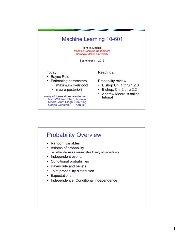
Probability Overview Random variables Axioms of probability What - PDF document

Machine Learning 10-601 Tom M. Mitchell Machine Learning Department Carnegie Mellon University September 11, 2012 Today: Readings: • Bayes Rule • Estimating parameters Probability review • maximum likelihood • Bishop Ch. 1 thru 1.2.3 • max a posteriori • Bishop, Ch. 2 thru 2.2 • Andrew Moore ’ s online many of these slides are derived tutorial from William Cohen, Andrew Moore, Aarti Singh, Eric Xing, Carlos Guestrin. - Thanks! Probability Overview • Random variables • Axioms of probability – What defines a reasonable theory of uncertainty • Independent events • Conditional probabilities • Bayes rule and beliefs • Joint probability distribution • Expectations • Independence, Conditional independence 1

Random Variables • Informally, A is a random variable if – A denotes something about which we are uncertain – perhaps the outcome of a randomized experiment • Examples A = True if a randomly drawn person from our class is female A = The hometown of a randomly drawn person from our class A = True if two randomly drawn persons from our class have same birthday • Define P(A) as “ the fraction of possible worlds in which A is true ” or “ the fraction of times A holds, in repeated runs of the random experiment ” – the set of possible worlds is called the sample space, S – A random variable A is a function defined over S A: S à {0,1} Visualizing Probabilities A ^ B Sample space of all possible worlds A B Its area is 1 2

The Axioms of Probability • 0 <= P(A) <= 1 • P(True) = 1 • P(False) = 0 • P(A or B) = P(A) + P(B) - P(A and B) [di Finetti 1931]: when gambling based on “ uncertainty formalism X ” you can be exploited by an opponent iff your uncertainty formalism X violates these axioms Useful theorems follow from the axioms Axioms: 0 <= P(A) <= 1, P(True) = 1, P(False) = 0, P(A or B) = P(A) + P(B) - P(A and B) * è P(A) = P(A ^ B) + P(A ^ ~B) A = [A and (B or ~B)] = [(A and B) or (A and ~B)] P(A) = P(A and B) + P(A and ~B) – P((A and B) and (A and ~B)) P(A) = P(A and B) + P(A and ~B) – P(A and B and A and ~B) * ¡Law ¡of ¡total ¡probability ¡ 3

Elementary Probability in Pictures • P(A) = P(A ^ B) + P(A ^ ~B) A ^ B A ^ ~B A B Definition of Conditional Probability P(A ^ B) P(A|B) = ----------- P(B) A B 4

Definition of Conditional Probability P(A ^ B) P(A|B) = ----------- P(B) Corollary: The Chain Rule P(A ^ B) = P(A|B) P(B) P(C ^ A ^ B) = P(C|A ^ B) P(A|B) P(B) Independent Events • Definition: two events A and B are independent if P(A ^ B)= P(A) P(B) • Intuition: knowing value of A tells us nothing about the value of B (and vice versa) 5

Picture “ A independent of B ” Bayes Rule • lets write 2 expressions for P(A ^ B) A ^ B A B 6

P(B|A) * P(A) Bayes ’ rule P(A|B) = P(B) we call P(A) the “ prior ” Bayes, Thomas (1763) An essay towards solving a problem in the doctrine and P(A|B) the “ posterior ” of chances. Philosophical Transactions of the Royal Society of London, 53:370-418 … by no means merely a curious speculation in the doctrine of chances, but necessary to be solved in order to a sure foundation for all our reasonings concerning past facts, and what is likely to be hereafter … . necessary to be considered by any that would give a clear account of the strength of analogical or inductive reasoning … Other Forms of Bayes Rule P ( B | A ) P ( A ) P ( A | B ) = P ( B | A ) P ( A ) P ( B |~ A ) P (~ A ) + P ( B | A X ) P ( A X ) ∧ ∧ P ( A | B X ) ∧ = P ( B X ) ∧ 7

Applying Bayes Rule P ( B | A ) P ( A ) P ( A | B ) = P ( B | A ) P ( A ) + P ( B |~ A ) P (~ A ) A = you have the flu, B = you just coughed Assume: P(flu) = 0.05 P(cough | flu) = 0.80 P(cough | ~flu) = 0.2 what is P(flu | cough)? what does all this have to do with function approximation? 8

The Joint Distribution Example: Boolean variables A, B, C A B C Prob Recipe for making a joint 0 0 0 0.30 distribution of M variables: 0 0 1 0.05 0 1 0 0.10 0 1 1 0.05 1 0 0 0.05 1 0 1 0.10 1 1 0 0.25 1 1 1 0.10 A 0.05 0.10 0.05 0.10 0.25 0.05 C 0.10 B 0.30 [A. Moore] The Joint Distribution Example: Boolean variables A, B, C A B C Prob Recipe for making a joint 0 0 0 0.30 distribution of M variables: 0 0 1 0.05 0 1 0 0.10 1. Make a truth table listing all 0 1 1 0.05 1 0 0 0.05 combinations of values of 1 0 1 0.10 your variables (if there are 1 1 0 0.25 M Boolean variables then 1 1 1 0.10 the table will have 2 M rows). A 0.05 0.10 0.05 0.10 0.25 0.05 C 0.10 B 0.30 [A. Moore] 9

The Joint Distribution Example: Boolean variables A, B, C A B C Prob Recipe for making a joint 0 0 0 0.30 distribution of M variables: 0 0 1 0.05 0 1 0 0.10 1. Make a truth table listing all 0 1 1 0.05 1 0 0 0.05 combinations of values of 1 0 1 0.10 your variables (if there are 1 1 0 0.25 M Boolean variables then 1 1 1 0.10 the table will have 2 M rows). 2. For each combination of A 0.05 0.10 0.05 values, say how probable it 0.10 is. 0.25 0.05 C 0.10 B 0.30 [A. Moore] The Joint Distribution Example: Boolean variables A, B, C A B C Prob Recipe for making a joint 0 0 0 0.30 distribution of M variables: 0 0 1 0.05 0 1 0 0.10 1. Make a truth table listing all 0 1 1 0.05 1 0 0 0.05 combinations of values of 1 0 1 0.10 your variables (if there are 1 1 0 0.25 M Boolean variables then 1 1 1 0.10 the table will have 2 M rows). 2. For each combination of A 0.05 0.10 0.05 values, say how probable it 0.10 is. 0.25 0.05 C 3. If you subscribe to the 0.10 axioms of probability, those B 0.30 numbers must sum to 1. [A. Moore] 10

Using the Joint One you have the JD P ( E ) P ( row ) ∑ = you can ask for the rows matching E probability of any logical expression involving your attribute [A. Moore] Using the Joint P(Poor Male) = 0.4654 P ( E ) P ( row ) ∑ = rows matching E [A. Moore] 11

Using the Joint P(Poor) = 0.7604 P ( E ) P ( row ) ∑ = rows matching E [A. Moore] Inference with the Joint P ( row ) ∑ P ( E E ) ∧ rows matching E and E P ( E | E ) 1 2 1 2 = = 1 2 P ( E ) P ( row ) ∑ 2 rows matching E 2 P(Male | Poor) = 0.4654 / 0.7604 = 0.612 [A. Moore] 12

Learning and the Joint Distribution Suppose we want to learn the function f: <G, H> à W Equivalently, P(W | G, H) Solution: learn joint distribution from data, calculate P(W | G, H) e.g., P(W=rich | G = female, H = 40.5- ) = [A. Moore] sounds like the solution to learning F: X à Y, or P(Y | X). Are we done? 13

[C. Guestrin] [C. Guestrin] 14

[C. Guestrin] Maximum Likelihood Estimate for Θ [C. Guestrin] 15

[C. Guestrin] [C. Guestrin] 16

[C. Guestrin] Beta prior distribution – P( θ ) [C. Guestrin] 17

Beta prior distribution – P( θ ) [C. Guestrin] [C. Guestrin] 18

[C. Guestrin] Conjugate priors [A. Singh] 19

Dirichlet distribution • number of heads in N flips of a two-sided coin – follows a binomial distribution – Beta is a good prior (conjugate prior for binomial) • what it ’ s not two-sided, but k-sided? – follows a multinomial distribution – Dirichlet distribution is the conjugate prior Conjugate priors [A. Singh] 20

Estimating Parameters • Maximum Likelihood Estimate (MLE): choose θ that maximizes probability of observed data • Maximum a Posteriori (MAP) estimate: choose θ that is most probable given prior probability and the data You should know • Probability basics – random variables, events, sample space, conditional probs, … – independence of random variables – Bayes rule – Joint probability distributions – calculating probabilities from the joint distribution • Estimating parameters from data – maximum likelihood estimates – maximum a posteriori estimates – distributions – binomial, Beta, Dirichlet, … – conjugate priors 21

Extra slides Expected values Given discrete random variable X, the expected value of X, written E[X] is We also can talk about the expected value of functions of X 22

Covariance Given two random vars X and Y, we define the covariance of X and Y as e.g., X=gender, Y=playsFootball or X=gender, Y=leftHanded Remember: [E. Xing] 23