CSE 573: Artificial Intelligence Bayes Net Teaser Gagan Bansal - PowerPoint PPT Presentation
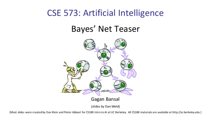
CSE 573: Artificial Intelligence Bayes Net Teaser Gagan Bansal (slides by Dan Weld) [Most slides were created by Dan Klein and Pieter Abbeel for CS188 Intro to AI at UC Berkeley. All CS188 materials are available at http://ai.berkeley.edu.]
CSE 573: Artificial Intelligence Bayes’ Net Teaser Gagan Bansal (slides by Dan Weld) [Most slides were created by Dan Klein and Pieter Abbeel for CS188 Intro to AI at UC Berkeley. All CS188 materials are available at http://ai.berkeley.edu.]
Probability Recap § Conditional probability § Product rule § Chain rule § Bayes rule § X, Y independent if and only if: § X and Y are conditionally independent given Z: if and only if:
Probabilistic Inference § Probabilistic inference = “compute a desired probability from other known probabilities (e.g. conditional from joint)” § We generally compute conditional probabilities § P(on time | no reported accidents) = 0.90 § These represent the agent’s beliefs given the evidence § Probabilities change with new evidence: § P(on time | no accidents, 5 a.m.) = 0.95 § P(on time | no accidents, 5 a.m., raining) = 0.80 § Observing new evidence causes beliefs to be updated
Inference by Enumeration * Works fine with General case: We want: § § multiple query Evidence variables: § variables, too Query* variable: § All variables Hidden variables: § Step 3: Normalize Step 1: Select the Step 2: Sum out H to get joint § § § entries consistent of Query and evidence with the evidence × 1 Z
Inference by Enumeration § Computational problems? § Worst-case time complexity O(d n ) § Space complexity O(d n ) to store the joint distribution
The Sword of Conditional Independence! Slay I am a BIG joint the distribution! Basilisk! harrypotter.wikia.com/ Means: Or, equivalently: 6
Bayes’Nets: Big Picture
Bayes’ Nets § Representation & Semantics § Conditional Independences § Probabilistic Inference § Learning Bayes’ Nets from Data
Bayes Nets = a Kind of Probabilistic Graphical Model § Models describe how (a portion of) the world works § Models are always simplifications § May not account for every variable § May not account for all interactions between variables § “All models are wrong; but some are useful.” – George E. P. Box Friction, § What do we do with probabilistic models? Air friction, § We (or our agents) need to reason about unknown variables, given evidence Mass of pulley, § Example: explanation (diagnostic reasoning) Inelastic string, … § Example: prediction (causal reasoning) § Example: value of information
Bayes’ Nets: Big Picture § Two problems with using full joint distribution tables as our probabilistic models: § Unless there are only a few variables, the joint is WAY too big to represent explicitly § Hard to learn (estimate) anything empirically about more than a few variables at a time § Bayes’ nets: a technique for describing complex joint distributions (models) using simple, local distributions (conditional probabilities) § More properly … aka probabilistic graphical model § We describe how variables locally interact § Local interactions chain together to give global, indirect interactions § For about 10 min, we’ll be vague about how these interactions are specified
Example Bayes’ Net: Insurance
Bayes’ Net Semantics
Bayes’ Net Semantics § A set of nodes, one per variable X P(A 1 ) …. P(A n ) A 1 A n § A directed, acyclic graph § A conditional distribution for each node § A collection of distributions over X, one for each X combination of parents’ values § CPT: conditional probability table § Description of a noisy “causal” process A Bayes net = Topology (graph) + Local Conditional Probabilities
Example: Alarm Network E P(E) B P(B) B urglary E arthqk +e 0.002 +b 0.001 -e 0.998 -b 0.999 A larm B E A P(A|B,E) +b +e +a 0.95 J ohn M ary +b +e -a 0.05 calls calls +b -e +a 0.94 A J P(J|A) A M P(M|A) +b -e -a 0.06 -b +e +a 0.29 +a +j 0.9 +a +m 0.7 -b +e -a 0.71 +a -j 0.1 +a -m 0.3 -b -e +a 0.001 -a +j 0.05 -a +m 0.01 -b -e -a 0.999 -a -j 0.95 -a -m 0.99
Bayes Nets Implicitly Encode Joint Distribution B P(B) E P(E) B E +b 0.001 +e 0.002 -b 0.999 -e 0.998 A A J P(J|A) A M P(M|A) B E A P(A|B,E) +a +j 0.9 +a +m 0.7 +b +e +a 0.95 +a -j 0.1 +a -m 0.3 J M +b +e -a 0.05 -a +j 0.05 -a +m 0.01 +b -e +a 0.94 -a -j 0.95 -a -m 0.99 +b -e -a 0.06 -b +e +a 0.29 -b +e -a 0.71 -b -e +a 0.001 -b -e -a 0.999
Bayes Nets Implicitly Encode Joint Distribution B P(B) E P(E) B E +b 0.001 +e 0.002 -b 0.999 -e 0.998 A A J P(J|A) A M P(M|A) B E A P(A|B,E) +a +j 0.9 +a +m 0.7 +b +e +a 0.95 +a -j 0.1 +a -m 0.3 J M +b +e -a 0.05 -a +j 0.05 -a +m 0.01 +b -e +a 0.94 -a -j 0.95 -a -m 0.99 +b -e -a 0.06 -b +e +a 0.29 -b +e -a 0.71 -b -e +a 0.001 -b -e -a 0.999
Joint Probabilities from BNs § Why are we guaranteed that setting results in a proper joint distribution? § Chain rule (valid for all distributions): § Assume conditional independences: à Consequence: § Every BN represents a joint distribution, but § Not every distribution can be represented by a specific BN § The topology enforces certain conditional independencies
Causality? § When Bayes’ nets reflect the true causal patterns: § Often simpler (nodes have fewer parents) § Often easier to think about § Often easier to elicit from experts § BNs need not actually be causal § Sometimes no causal net exists over the domain (especially if variables are missing) § E.g. consider the variables Traffic and Drips § End up with arrows that reflect correlation, not causation § What do the arrows really mean? § Topology may happen to encode causal structure § Topology really encodes conditional independence
Size of a Bayes ’ Net § How big is a joint distribution over N § Both give you the power to calculate Boolean variables? 2 N § BNs: Huge space savings! § How big is an N-node net if nodes § Also easier to elicit local CPTs have up to k parents? O(N * 2 k ) § Also faster to answer queries (coming)
Inference in Bayes’ Net § Many algorithms for both exact and approximate inference § Complexity often based on § Structure of the network § Size of undirected cycles § Usually faster than exponential in number of nodes Exact inference § § Variable elimination § Junction trees and belief propagation § Approximate inference § Loopy belief propagation § Sampling based methods: likelihood weighting, Markov chain Monte Carlo § Variational approximation
Summary: Bayes ’ Net Semantics § A directed, acyclic graph, one node per random variable § A conditional probability table (CPT) for each node § A collection of distributions over X, one for each combination of parents ’ values § Bayes ’ nets compactly encode joint distributions § As a product of local conditional distributions § To see what probability a BN gives to a full assignment, multiply all the relevant conditionals together:
Hidden Markov Models X 1 X 2 X 3 X 4 X N X 5 E 1 E 2 E 3 E 4 E N E 5 § Defines a joint probability distribution:
Hidden Markov Models X 1 X 2 X 3 X 4 X N X 5 E 1 E 2 E 3 E 4 E N E 5 § An HMM is defined by: § Initial distribution: § Transitions: § Emissions:
Conditional Independence HMMs have two important independence properties: § Future independent of past given the present ? ? X 1 X 2 X 3 X 4 E 1 E 2 E 3 E 4
Conditional Independence HMMs have two important independence properties: § Future independent of past given the present § Current observation independent of all else given current state ? X 1 X 2 X 3 X 4 E 1 E 2 E 3 E 4 ?
Conditional Independence § HMMs have two important independence properties: § Markov hidden process, future depends on past via the present § Current observation independent of all else given current state X 1 X 2 X 3 X 4 E 1 E 2 E 3 E 4 ? ? § Quiz: does this mean that observations are independent given no evidence? § [No, correlated by the hidden state]
Inference in Ghostbusters § A ghost is in the grid somewhere § Sensor readings tell how close a square is to the ghost § On the ghost: red § 1 or 2 away: orange § 3 or 4 away: yellow § 5+ away: green § Sensors are noisy, but we know P(Color | Distance) P(red | 3) P(orange | 3) P(yellow | 3) P(green | 3) 0.05 0.15 0.5 0.3 [Demo: Ghostbuster – no probability (L12D1) ]
Ghostbusters HMM § P(X 1 ) = uniform 1/9 1/9 1/9 § P(X’|X) = ghosts usually move clockwise, 1/9 1/9 1/9 but sometimes move in a random direction or stay put 1/9 1/9 1/9 § P(E|X) = same sensor model as before: red means probably close, green means likely far away. P(X 1 ) 1/6 1/6 1/2 X 1 X 2 X 3 X 4 0 1/6 0 Etc… 0 0 0 E 1 E 2 E 3 E 4 P(X’|X=<1,2>) P(E|X) X P(red | x) P(orange | x) P(yellow | x) P(green | x) (One row 2 … … … … for every E 5 value of X) 3 0.05 0.15 0.5 0.3 4 … … … …
HMM Examples § Speech recognition HMMs: § States are specific positions in specific words (so, tens of thousands ) § Observations are acoustic signals (continuous valued) X 1 X 2 X 3 X 4 E 1 E 2 E 3 E 4
HMM Examples § POS tagging HMMs: § State is the parts of speech tag for a specific word § Observations are words in a sentence (size of the vocabulary) X 1 X 2 X 3 X 4 E 1 E 2 E 3 E 4
Recommend
More recommend
Explore More Topics
Stay informed with curated content and fresh updates.
