CSE 573: Artificial Intelligence Reinforcement Learning Dan Weld/ - PowerPoint PPT Presentation
CSE 573: Artificial Intelligence Reinforcement Learning Dan Weld/ University of Washington [Many slides taken from Dan Klein and Pieter Abbeel / CS188 Intro to AI at UC Berkeley materials available at http://ai.berkeley.edu.] Logistics Title
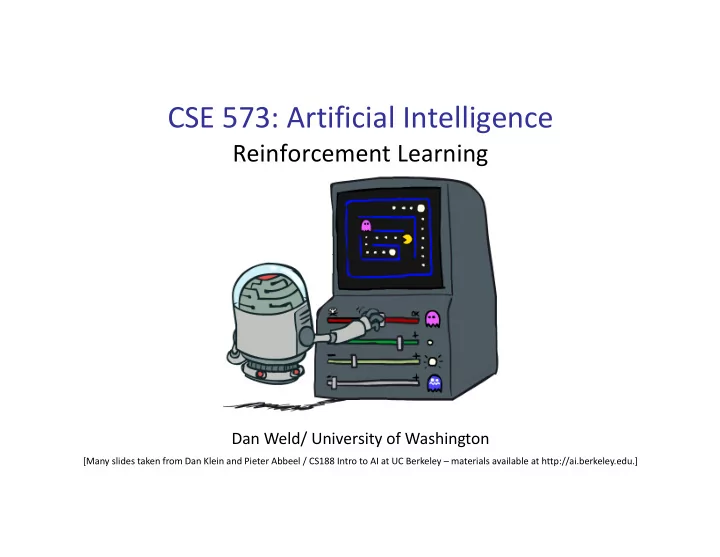
CSE 573: Artificial Intelligence Reinforcement Learning Dan Weld/ University of Washington [Many slides taken from Dan Klein and Pieter Abbeel / CS188 Intro to AI at UC Berkeley – materials available at http://ai.berkeley.edu.]
Logistics Title : Neural Question Answering over Knowledge Graphs Speaker : Wenpeng Yin (University of Munich) Time : Thursday, Feb 16, 10:30 am Location : CSE 403 2
Offline (MDPs) vs. Online (RL) Simulator Offline Solution Monte Carlo Online Learning (Planning) Planning (RL) Diff: 1) dying ok; 2) (re)set button
Approximate Q Learning § Forall i § Initialize w i = 0 § Repeat Forever Where are you? s. Choose some action a Execute it in real world: (s, a, r, s’) Do update: difference ß [r + γ Max a’ Q(s’, a’)] - Q(s,a) Forall i do:
Exploration vs. Exploitation
Two KINDS of Regret § Cumulative Regret: § achieve near optimal cumulative lifetime reward (in expectation) § Simple Regret: § quickly identify policy with high reward (in expectation) 107
Regret Reward ∞ Time Exploration policy that minimizes cumulative regret Minimizes red area 108
Regret Reward ∞ t Time Exploration policy that minimizes simple regret… For any time, t, minimizes red area after t 109
RL on Single State MDP § Suppose MDP has a single state and k actions § Can sample rewards of actions using call to simulator § Sampling action a is like pulling slot machine arm with random payoff function R ( s , a ) s a k a 1 a 2 … … R(s,a 2 ) R(s,a k ) R(s,a 1 ) Multi-Armed Bandit Problem 110 Slide adapted from Alan Fern (OSU)
Cumulative Regret Objective h Problem: find arm-pulling strategy such that the expected total reward at time n is close to the best possible (one pull per time step) 5 Optimal (in expectation) is to pull optimal arm n times 5 UniformBandit is poor choice --- waste time on bad arms 5 Must balance exploring machines to find good payoffs and exploiting current knowledge s a k a 1 a 2 … 116 Slide adapted from Alan Fern (OSU)
� Idea • The problem is uncertainty… How to quantify? • Error bars If arm has been sampled n times, With probability at least 1- 𝜀 : (2 log 𝜀) 𝜈 " − 𝜈 < 2𝑜 Slide adapted from Travis Mandel (UW)
Given Error bars, how do we act? • Optimism under uncertainty! • Why? If bad, we will soon find out! Slide adapted from Travis Mandel (UW)
� Upper Confidence Bound (UCB) 1. Play each arm once 2. Play arm i that maximizes: 2log (𝑢) 𝜈 " / + 𝑜 / 3. Repeat Step 2 forever Slide adapted from Travis Mandel (UW)
UCB Performance Guarantee [Auer, Cesa-Bianchi, & Fischer, 2002] Theorem : The expected cumulative regret of UCB 𝑭[𝑺𝒇𝒉 𝒐 ] after n arm pulls is bounded by O(log n ) 𝑭[𝑺𝒇𝒉 𝒐 ] 𝑭[𝑺𝒇𝒉 𝒐 ] � Is this good? � � log 𝑜 Yes. The average per-step regret is O log 𝑜 log 𝑜 𝑜 𝑜 𝑜 Theorem: No algorithm can achieve a better expected regret (up to constant factors) 125 Slide adapted from Alan Fern (OSU)
UCB as Exploration Function in Q-Learning Σ Let N sa be number of times one has executed a in s; let N = N sa sa Let Q e (s,a) = Q(s,a) + √ log(N)/(1+n sa ) § Forall s, a § Initialize Q(s, a) = 0, n sa = 0 § Repeat Forever Where are you? s. Choose action with highest Q e Execute it in real world: (s, a, r, s’) Do update: N sa += 1; difference ß [r + γ Max a’ Q e (s’, a’)] - Q e (s,a) Q(s,a) ß Q e (s,a) + 𝛽 (difference) 126
Video of Demo Q-learning – Epsilon-Greedy – Crawler
Video of Demo Q-learning – Exploration Function – Crawler
A little history… William R. Thompson (1933): Was the first to examine MAB problem, proposed a method for solving them 1940s-50s: MAB problem studied intentively during WWII, Thompson was ignored 1970’s-1980’s: “Optimal” solution (Gittins index) found but is intractable and incomplete. Thompson ignored. 2001: UCB proposed, gains widespread use due to simplicity and “optimal” bounds. Thompson still ignored. 2011: Empricial results show Thompson’s 1933 method beats UCB, but little interest since no guarantees. 2013: Optimal bounds finally shown for Thompson Sampling Slide adapted from Travis Mandel (UW)
Thompson’s method was fundamentally different!
Bayesian vs. Frequentist • Bayesians: You have a prior, probabilities interpreted as beliefs, prefer probabilistic decisions • Frequentists: No prior, probabilities interpreted as facts about the world, prefer hard decisions (p<0.05) UCB is a frequentist technique! What if we are Bayesian?
Bayesian review: Bayes’ Rule 𝑞 𝜄 𝑒𝑏𝑢𝑏) = 𝑞 𝑒𝑏𝑢𝑏 𝜄 𝑞(𝜄) 𝑞(𝑒𝑏𝑢𝑏) Posterior 𝑞 𝜄 𝑒𝑏𝑢𝑏) ∝ 𝑞 𝑒𝑏𝑢𝑏 𝜄 𝑞(𝜄) Likelihood Prior
Bernoulli Case What if distribution in the set {0,1} instead of the range [0,1] ? Then we flip a coin with probability p à Bernoulli distribution! To estimate p, we count up numbers of ones and zeros Given observed ones and zeroes, how do we calculate the distribution of possible values of p?
Beta-Bernoulli Case Beta(a,b) à Given a 0’s and b 1’s, what is the distribution over means? Prior à pseudocounts Likelihood à Observed counts Posterior à pseudocounts + observed counts
How does this help us? Thompson Sampling: 1. Specify prior (e.g., using Beta(1,1)) 2. Sample from each posterior distribution to get estimated mean for each arm. 3. Pull arm with highest mean. 4. Repeat step 2 & 3 forever
Thompson Empirical Results And shown to have optimal regret bounds just like (and in some cases a little better than) UCB!
What Else …. h UCB & Thompson is great when we care about cumulative regret h I.e., when the agent is acting in the real world h But, sometimes all we care about is finding a good arm quickly h E.g., when we are training in a simulator h In these cases, “Simple Regret” is better objective 137
Two KINDS of Regret § Cumulative Regret: § achieve near optimal cumulative lifetime reward (in expectation) § Simple Regret: § quickly identify policy with high reward (in expectation) 138
Simple Regret Objective � � Protocol: At time step n the algorithm picks an “exploration” arm 𝑏 𝑜 𝑠 𝑘 𝑜 “exploration” arm 𝑏 𝑜 to pull and observes reward 𝑜 𝑠 𝑜 and also picks an arm index it thinks is best 𝑘 𝑜 𝑏 𝑜 , 𝑘 𝑜 and 𝑠 𝑜 ( 𝑏 𝑜 , 𝑘 𝑜 and 𝑠 𝑜 are random variables) . 𝑘 𝑜 � � If interrupted at time n the algorithm returns 𝑘 𝑜 . � Expected Simple Regret ( 𝑭[𝑻𝑺𝒇𝒉 𝒐 ]) : difference between 𝑆 ∗ and expected reward of arm 𝑘 𝑜 𝑭[𝑻𝑺𝒇𝒉 𝒐 ]) � selected by our strategy at time n 𝑆 ∗ 𝑘 𝑜 𝐹[𝑇𝑆𝑓 𝑜 ] = 𝑆 ∗ − 𝐹[𝑆(𝑏 𝑘 𝑜 )] 𝐹[𝑇𝑆𝑓 𝑜 ] = 𝑆 ∗ − 𝐹[𝑆(𝑏 𝑘 𝑜 )] 139
� � How to Minimize Simple Regret? � What about UCB for simple regret? Theorem : The expected simple regret of UCB after n arm pulls is upper bounded by O 𝑜 −𝑑 for a constant c. Seems good, but we can do much better (at least in theory). Ø Intuitively: UCB puts too much emphasis on pulling the best arm Ø After an arm is looking good, maybe better to see if ∃ a better arm
Incremental Uniform (or Round Robin) Bubeck, S., Munos, R., & Stoltz, G. (2011). Pure exploration in finitely-armed and continuous-armed bandits. Theoretical Computer Science, 412(19), 1832-1852 Algorithm: � � � At round n pull arm with index (k mod n) + 1 � � � At round n return arm (if asked) with largest average reward Theorem : The expected simple regret of Uniform after n arm pulls is upper bounded by O 𝑓 −𝑑𝑜 for a constant c. 𝑓 −𝑑𝑜 𝑓 −𝑑𝑜 � � This bound is exponentially decreasing in n! � 𝑜 −𝑑 Compared to polynomially for UCB O 𝑜 −𝑑 . 𝑜 −𝑑 141
Can we do even better? Tolpin, D. & Shimony, S, E. (2012). MCTS Based on Simple Regret. AAAI Conference on Artificial Intelligence. Algorithm -Greedy : (parameter ) 𝜗 0 < 𝜗 < 1 § At round n, with probability pull arm with best average reward so far, otherwise pull one of the other arms at random. 𝜗 � § At round n return arm (if asked) with largest average reward � Theorem : The expected simple regret of 𝜗 - Greedy for 𝜗 = 0.5 after n arm pulls is upper bounded by O 𝑓 −𝑑𝑜 for a constant c that is larger than the constant for Uniform (this holds for “large enough” n). 142
Summary of Bandits in Theory PAC Objective: UniformBandit is a simple PAC algorithm § MedianElimination improves by a factor of log(k) and is optimal up to § constant factors Cumulative Regret: Uniform is very bad! § UCB is optimal (up to constant factors) § Thomson Sampling also optimal; often performs better in practice § Simple Regret: UCB shown to reduce regret at polynomial rate § Uniform reduces at an exponential rate § 0.5-Greedy may have even better exponential rate §
Theory vs . Practice The established theoretical relationships among bandit • algorithms have often been useful in predicting empirical relationships. But not always …. •
Recommend
More recommend
Explore More Topics
Stay informed with curated content and fresh updates.

