Probabilistic & Unsupervised Learning Expectation Maximisation - PowerPoint PPT Presentation
Probabilistic & Unsupervised Learning Expectation Maximisation Maneesh Sahani maneesh@gatsby.ucl.ac.uk Gatsby Computational Neuroscience Unit, and MSc ML/CSML, Dept Computer Science University College London Term 1, Autumn 2018
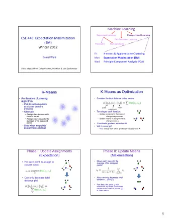
The Expectation Maximisation (EM) algorithm The EM algorithm (Dempster, Laird & Rubin, 1977; but significant earlier precedents) finds a (local) maximum of a latent variable model likelihood. Start from arbitrary values of the parameters, and iterate two steps: E step: Fill in values of latent variables according to posterior given data. M step: Maximise likelihood as if latent variables were not hidden. ◮ Decomposes difficult problems into series of tractable steps. ◮ An alternative to gradient-based iterative methods. ◮ No learning rate. ◮ In ML, the E step is called inference, and the M step learning. In stats, these are often imputation and inference or estimation. ◮ Not essential for simple models (like MoGs/FA), though often more efficient than alternatives. Crucial for learning in complex settings.
The Expectation Maximisation (EM) algorithm The EM algorithm (Dempster, Laird & Rubin, 1977; but significant earlier precedents) finds a (local) maximum of a latent variable model likelihood. Start from arbitrary values of the parameters, and iterate two steps: E step: Fill in values of latent variables according to posterior given data. M step: Maximise likelihood as if latent variables were not hidden. ◮ Decomposes difficult problems into series of tractable steps. ◮ An alternative to gradient-based iterative methods. ◮ No learning rate. ◮ In ML, the E step is called inference, and the M step learning. In stats, these are often imputation and inference or estimation. ◮ Not essential for simple models (like MoGs/FA), though often more efficient than alternatives. Crucial for learning in complex settings. ◮ Provides a framework for principled approximations.
Jensen’s inequality One view: EM iteratively refines a lower bound on the log-likelihood.
Jensen’s inequality One view: EM iteratively refines a lower bound on the log-likelihood. log ( x ) x 1 x 2
Jensen’s inequality One view: EM iteratively refines a lower bound on the log-likelihood. log ( x ) x 1 x 2
Jensen’s inequality One view: EM iteratively refines a lower bound on the log-likelihood. log ( x ) α x 1 + ( 1 − α ) x 2 x 1 x 2
Jensen’s inequality One view: EM iteratively refines a lower bound on the log-likelihood. log ( x ) log ( α x 1 + ( 1 − α ) x 2 ) α log ( x 1 ) + ( 1 − α ) log ( x 2 ) α x 1 + ( 1 − α ) x 2 x 1 x 2
Jensen’s inequality One view: EM iteratively refines a lower bound on the log-likelihood. log ( x ) log ( α x 1 + ( 1 − α ) x 2 ) α log ( x 1 ) + ( 1 − α ) log ( x 2 ) α x 1 + ( 1 − α ) x 2 x 1 x 2 In general:
Jensen’s inequality One view: EM iteratively refines a lower bound on the log-likelihood. log ( x ) log ( α x 1 + ( 1 − α ) x 2 ) α log ( x 1 ) + ( 1 − α ) log ( x 2 ) α x 1 + ( 1 − α ) x 2 x 1 x 2 In general: For α i ≥ 0, � α i = 1 (and { x i > 0 } ) : � � � � α i x i ≥ α i log ( x i ) log i i
Jensen’s inequality One view: EM iteratively refines a lower bound on the log-likelihood. log ( x ) log ( α x 1 + ( 1 − α ) x 2 ) α log ( x 1 ) + ( 1 − α ) log ( x 2 ) α x 1 + ( 1 − α ) x 2 x 1 x 2 In general: For α i ≥ 0, � α i = 1 (and { x i > 0 } ) : For probability measure α and concave f � � � � α i x i ≥ α i log ( x i ) f ( E α [ x ]) ≥ E α [ f ( x )] log i i
Jensen’s inequality One view: EM iteratively refines a lower bound on the log-likelihood. log ( x ) log ( α x 1 + ( 1 − α ) x 2 ) α log ( x 1 ) + ( 1 − α ) log ( x 2 ) α x 1 + ( 1 − α ) x 2 x 1 x 2 In general: For α i ≥ 0, � α i = 1 (and { x i > 0 } ) : For probability measure α and concave f � � � � α i x i ≥ α i log ( x i ) f ( E α [ x ]) ≥ E α [ f ( x )] log i i Equality (if and) only if f ( x ) is almost surely constant or linear on (convex) support of α .
The lower bound for EM – “free energy” Observed data X = { x i } ; Latent variables Z = { z i } ; Parameters θ = { θ x , θ z } . � Log-likelihood: ℓ ( θ ) = log P ( X| θ ) = log d Z P ( Z , X| θ )
The lower bound for EM – “free energy” Observed data X = { x i } ; Latent variables Z = { z i } ; Parameters θ = { θ x , θ z } . � Log-likelihood: ℓ ( θ ) = log P ( X| θ ) = log d Z P ( Z , X| θ ) By Jensen, any distribution, q ( Z ) , over the latent variables generates a lower bound: � d Z P ( Z , X| θ ) ℓ ( θ ) = log
The lower bound for EM – “free energy” Observed data X = { x i } ; Latent variables Z = { z i } ; Parameters θ = { θ x , θ z } . � Log-likelihood: ℓ ( θ ) = log P ( X| θ ) = log d Z P ( Z , X| θ ) By Jensen, any distribution, q ( Z ) , over the latent variables generates a lower bound: � d Z q ( Z ) P ( Z , X| θ ) ℓ ( θ ) = log q ( Z )
The lower bound for EM – “free energy” Observed data X = { x i } ; Latent variables Z = { z i } ; Parameters θ = { θ x , θ z } . � Log-likelihood: ℓ ( θ ) = log P ( X| θ ) = log d Z P ( Z , X| θ ) By Jensen, any distribution, q ( Z ) , over the latent variables generates a lower bound: � � d Z q ( Z ) P ( Z , X| θ ) d Z q ( Z ) log P ( Z , X| θ ) ≥ ℓ ( θ ) = log q ( Z ) q ( Z )
The lower bound for EM – “free energy” Observed data X = { x i } ; Latent variables Z = { z i } ; Parameters θ = { θ x , θ z } . � Log-likelihood: ℓ ( θ ) = log P ( X| θ ) = log d Z P ( Z , X| θ ) By Jensen, any distribution, q ( Z ) , over the latent variables generates a lower bound: � � d Z q ( Z ) P ( Z , X| θ ) d Z q ( Z ) log P ( Z , X| θ ) def ≥ = F ( q , θ ) . ℓ ( θ ) = log q ( Z ) q ( Z )
The lower bound for EM – “free energy” Observed data X = { x i } ; Latent variables Z = { z i } ; Parameters θ = { θ x , θ z } . � Log-likelihood: ℓ ( θ ) = log P ( X| θ ) = log d Z P ( Z , X| θ ) By Jensen, any distribution, q ( Z ) , over the latent variables generates a lower bound: � � d Z q ( Z ) P ( Z , X| θ ) d Z q ( Z ) log P ( Z , X| θ ) def ≥ = F ( q , θ ) . ℓ ( θ ) = log q ( Z ) q ( Z ) Now, � � � d Z q ( Z ) log P ( Z , X| θ ) d Z q ( Z ) log P ( Z , X| θ ) − d Z q ( Z ) log q ( Z ) = q ( Z )
The lower bound for EM – “free energy” Observed data X = { x i } ; Latent variables Z = { z i } ; Parameters θ = { θ x , θ z } . � Log-likelihood: ℓ ( θ ) = log P ( X| θ ) = log d Z P ( Z , X| θ ) By Jensen, any distribution, q ( Z ) , over the latent variables generates a lower bound: � � d Z q ( Z ) P ( Z , X| θ ) d Z q ( Z ) log P ( Z , X| θ ) def ≥ = F ( q , θ ) . ℓ ( θ ) = log q ( Z ) q ( Z ) Now, � � � d Z q ( Z ) log P ( Z , X| θ ) d Z q ( Z ) log P ( Z , X| θ ) − d Z q ( Z ) log q ( Z ) = q ( Z ) � = d Z q ( Z ) log P ( Z , X| θ ) + H [ q ] , where H [ q ] is the entropy of q ( Z ) .
The lower bound for EM – “free energy” Observed data X = { x i } ; Latent variables Z = { z i } ; Parameters θ = { θ x , θ z } . � Log-likelihood: ℓ ( θ ) = log P ( X| θ ) = log d Z P ( Z , X| θ ) By Jensen, any distribution, q ( Z ) , over the latent variables generates a lower bound: � � d Z q ( Z ) P ( Z , X| θ ) d Z q ( Z ) log P ( Z , X| θ ) def ≥ = F ( q , θ ) . ℓ ( θ ) = log q ( Z ) q ( Z ) Now, � � � d Z q ( Z ) log P ( Z , X| θ ) d Z q ( Z ) log P ( Z , X| θ ) − d Z q ( Z ) log q ( Z ) = q ( Z ) � = d Z q ( Z ) log P ( Z , X| θ ) + H [ q ] , where H [ q ] is the entropy of q ( Z ) . So: F ( q , θ ) = � log P ( Z , X| θ ) � q ( Z ) + H [ q ]
The E and M steps of EM The free-energy lower bound on ℓ ( θ ) is a function of θ and a distribution q : F ( q , θ ) = � log P ( Z , X| θ ) � q ( Z ) + H [ q ] ,
The E and M steps of EM The free-energy lower bound on ℓ ( θ ) is a function of θ and a distribution q : F ( q , θ ) = � log P ( Z , X| θ ) � q ( Z ) + H [ q ] , The EM steps can be re-written: ◮ E step: optimize F ( q , θ ) wrt distribution over hidden variables holding parameters fixed: � q ( Z ) , θ ( k − 1 ) � q ( k ) ( Z ) := argmax F . q ( Z )
The E and M steps of EM The free-energy lower bound on ℓ ( θ ) is a function of θ and a distribution q : F ( q , θ ) = � log P ( Z , X| θ ) � q ( Z ) + H [ q ] , The EM steps can be re-written: ◮ E step: optimize F ( q , θ ) wrt distribution over hidden variables holding parameters fixed: � q ( Z ) , θ ( k − 1 ) � q ( k ) ( Z ) := argmax F . q ( Z ) ◮ M step: maximize F ( q , θ ) wrt parameters holding hidden distribution fixed: � � θ ( k ) := argmax q ( k ) ( Z ) , θ F � log P ( Z , X| θ ) � q ( k ) ( Z ) = argmax θ θ � � q ( k ) ( Z ) does not depend directly on θ . The second equality comes from the fact that H
The E Step The free energy can be re-written
The E Step The free energy can be re-written � q ( Z ) log P ( Z , X| θ ) F ( q , θ ) = d Z q ( Z )
The E Step The free energy can be re-written � q ( Z ) log P ( Z , X| θ ) F ( q , θ ) = d Z q ( Z ) � q ( Z ) log P ( Z|X , θ ) P ( X| θ ) = d Z q ( Z )
The E Step The free energy can be re-written � q ( Z ) log P ( Z , X| θ ) F ( q , θ ) = d Z q ( Z ) � q ( Z ) log P ( Z|X , θ ) P ( X| θ ) = d Z q ( Z ) � � q ( Z ) log P ( Z|X , θ ) = q ( Z ) log P ( X| θ ) d Z + d Z q ( Z )
The E Step The free energy can be re-written � q ( Z ) log P ( Z , X| θ ) F ( q , θ ) = d Z q ( Z ) � q ( Z ) log P ( Z|X , θ ) P ( X| θ ) = d Z q ( Z ) � � q ( Z ) log P ( Z|X , θ ) = q ( Z ) log P ( X| θ ) d Z + d Z q ( Z ) = ℓ ( θ ) − KL [ q ( Z ) � P ( Z|X , θ )] The second term is the Kullback-Leibler divergence.
The E Step The free energy can be re-written � q ( Z ) log P ( Z , X| θ ) F ( q , θ ) = d Z q ( Z ) � q ( Z ) log P ( Z|X , θ ) P ( X| θ ) = d Z q ( Z ) � � q ( Z ) log P ( Z|X , θ ) = q ( Z ) log P ( X| θ ) d Z + d Z q ( Z ) = ℓ ( θ ) − KL [ q ( Z ) � P ( Z|X , θ )] The second term is the Kullback-Leibler divergence. This means that, for fixed θ , F is bounded above by ℓ , and achieves that bound when KL [ q ( Z ) � P ( Z|X , θ )] = 0.
The E Step The free energy can be re-written � q ( Z ) log P ( Z , X| θ ) F ( q , θ ) = d Z q ( Z ) � q ( Z ) log P ( Z|X , θ ) P ( X| θ ) = d Z q ( Z ) � � q ( Z ) log P ( Z|X , θ ) = q ( Z ) log P ( X| θ ) d Z + d Z q ( Z ) = ℓ ( θ ) − KL [ q ( Z ) � P ( Z|X , θ )] The second term is the Kullback-Leibler divergence. This means that, for fixed θ , F is bounded above by ℓ , and achieves that bound when KL [ q ( Z ) � P ( Z|X , θ )] = 0. But KL [ q � p ] is zero if and only if q = p (see appendix.)
The E Step The free energy can be re-written � q ( Z ) log P ( Z , X| θ ) F ( q , θ ) = d Z q ( Z ) � q ( Z ) log P ( Z|X , θ ) P ( X| θ ) = d Z q ( Z ) � � q ( Z ) log P ( Z|X , θ ) = q ( Z ) log P ( X| θ ) d Z + d Z q ( Z ) = ℓ ( θ ) − KL [ q ( Z ) � P ( Z|X , θ )] The second term is the Kullback-Leibler divergence. This means that, for fixed θ , F is bounded above by ℓ , and achieves that bound when KL [ q ( Z ) � P ( Z|X , θ )] = 0. But KL [ q � p ] is zero if and only if q = p (see appendix.) So, the E step sets q ( k ) ( Z ) = P ( Z|X , θ ( k − 1 ) ) [inference / imputation] and, after an E step, the free energy equals the likelihood.
Coordinate Ascent in F (Demo) To visualise, we consider a one parameter / one latent mixture: s ∼ Bernoulli [ π ] x | s = 0 ∼ N [ − 1 , 1 ] x | s = 1 ∼ N [ 1 , 1 ] . Single data point x 1 = . 3. q ( s ) is a distribution on a single binary latent, and so is represented by r 1 ∈ [ 0 , 1 ] . 0.4 0.35 0.3 0.25 0.2 0.15 0.1 0.05 0 −2 −1.5 −1 −0.5 0 0.5 1 1.5 2
Coordinate Ascent in F (Demo)
Coordinate Ascent in F (Demo)
Coordinate Ascent in F (Demo)
Coordinate Ascent in F (Demo)
Coordinate Ascent in F (Demo)
Coordinate Ascent in F (Demo)
Coordinate Ascent in F (Demo)
Coordinate Ascent in F (Demo)
Coordinate Ascent in F (Demo)
Coordinate Ascent in F (Demo)
Coordinate Ascent in F (Demo)
Coordinate Ascent in F (Demo)
Coordinate Ascent in F (Demo)
Coordinate Ascent in F (Demo)
Coordinate Ascent in F (Demo)
Coordinate Ascent in F (Demo)
Coordinate Ascent in F (Demo)
Coordinate Ascent in F (Demo)
Coordinate Ascent in F (Demo)
Coordinate Ascent in F (Demo)
Coordinate Ascent in F (Demo)
Coordinate Ascent in F (Demo)
Coordinate Ascent in F (Demo)
Coordinate Ascent in F (Demo)
Coordinate Ascent in F (Demo)
EM Never Decreases the Likelihood The E and M steps together never decrease the log likelihood: � θ ( k − 1 ) � ℓ
EM Never Decreases the Likelihood The E and M steps together never decrease the log likelihood: � θ ( k − 1 ) � � q ( k ) , θ ( k − 1 ) � ℓ = F E step ◮ The E step brings the free energy to the likelihood.
EM Never Decreases the Likelihood The E and M steps together never decrease the log likelihood: � θ ( k − 1 ) � � q ( k ) , θ ( k − 1 ) � � q ( k ) , θ ( k ) � ℓ = F ≤ F E step M step ◮ The E step brings the free energy to the likelihood. ◮ The M-step maximises the free energy wrt θ .
EM Never Decreases the Likelihood The E and M steps together never decrease the log likelihood: � θ ( k − 1 ) � � q ( k ) , θ ( k − 1 ) � � q ( k ) , θ ( k ) � � θ ( k ) � ℓ = F ≤ F ≤ ℓ , E step M step Jensen ◮ The E step brings the free energy to the likelihood. ◮ The M-step maximises the free energy wrt θ . ◮ F ≤ ℓ by Jensen – or, equivalently, from the non-negativity of KL
EM Never Decreases the Likelihood The E and M steps together never decrease the log likelihood: � θ ( k − 1 ) � � q ( k ) , θ ( k − 1 ) � � q ( k ) , θ ( k ) � � θ ( k ) � ℓ = F ≤ F ≤ ℓ , E step M step Jensen ◮ The E step brings the free energy to the likelihood. ◮ The M-step maximises the free energy wrt θ . ◮ F ≤ ℓ by Jensen – or, equivalently, from the non-negativity of KL If the M-step is executed so that θ ( k ) � = θ ( k − 1 ) iff F increases, then the overall EM iteration will step to a new value of θ iff the likelihood increases.
EM Never Decreases the Likelihood The E and M steps together never decrease the log likelihood: � θ ( k − 1 ) � � q ( k ) , θ ( k − 1 ) � � q ( k ) , θ ( k ) � � θ ( k ) � ℓ = F ≤ F ≤ ℓ , E step M step Jensen ◮ The E step brings the free energy to the likelihood. ◮ The M-step maximises the free energy wrt θ . ◮ F ≤ ℓ by Jensen – or, equivalently, from the non-negativity of KL If the M-step is executed so that θ ( k ) � = θ ( k − 1 ) iff F increases, then the overall EM iteration will step to a new value of θ iff the likelihood increases. Can also show that fixed points of EM (generally) correspond to maxima of the likelihood (see appendices).
EM Summary ◮ An iterative algorithm that finds (local) maxima of the likelihood of a latent variable model. � ℓ ( θ ) = log P ( X| θ ) = log d Z P ( X|Z , θ ) P ( Z| θ )
EM Summary ◮ An iterative algorithm that finds (local) maxima of the likelihood of a latent variable model. � ℓ ( θ ) = log P ( X| θ ) = log d Z P ( X|Z , θ ) P ( Z| θ ) ◮ Increases a variational lower bound on the likelihood by coordinate ascent. F ( q , θ ) = � log P ( Z , X| θ ) � q ( Z ) + H [ q ] = ℓ ( θ ) − KL [ q ( Z ) � P ( Z|X )] ≤ ℓ ( θ )
EM Summary ◮ An iterative algorithm that finds (local) maxima of the likelihood of a latent variable model. � ℓ ( θ ) = log P ( X| θ ) = log d Z P ( X|Z , θ ) P ( Z| θ ) ◮ Increases a variational lower bound on the likelihood by coordinate ascent. F ( q , θ ) = � log P ( Z , X| θ ) � q ( Z ) + H [ q ] = ℓ ( θ ) − KL [ q ( Z ) � P ( Z|X )] ≤ ℓ ( θ ) ◮ E step: � q ( Z ) , θ ( k − 1 ) � q ( k ) ( Z ) := argmax = P ( Z|X , θ ( k − 1 ) ) F q ( Z )
EM Summary ◮ An iterative algorithm that finds (local) maxima of the likelihood of a latent variable model. � ℓ ( θ ) = log P ( X| θ ) = log d Z P ( X|Z , θ ) P ( Z| θ ) ◮ Increases a variational lower bound on the likelihood by coordinate ascent. F ( q , θ ) = � log P ( Z , X| θ ) � q ( Z ) + H [ q ] = ℓ ( θ ) − KL [ q ( Z ) � P ( Z|X )] ≤ ℓ ( θ ) ◮ E step: � q ( Z ) , θ ( k − 1 ) � q ( k ) ( Z ) := argmax = P ( Z|X , θ ( k − 1 ) ) F q ( Z ) ◮ M step: � � θ ( k ) := argmax q ( k ) ( Z ) , θ F = argmax � log P ( Z , X| θ ) � q ( k ) ( Z ) θ θ
EM Summary ◮ An iterative algorithm that finds (local) maxima of the likelihood of a latent variable model. � ℓ ( θ ) = log P ( X| θ ) = log d Z P ( X|Z , θ ) P ( Z| θ ) ◮ Increases a variational lower bound on the likelihood by coordinate ascent. F ( q , θ ) = � log P ( Z , X| θ ) � q ( Z ) + H [ q ] = ℓ ( θ ) − KL [ q ( Z ) � P ( Z|X )] ≤ ℓ ( θ ) ◮ E step: � q ( Z ) , θ ( k − 1 ) � q ( k ) ( Z ) := argmax = P ( Z|X , θ ( k − 1 ) ) F q ( Z ) ◮ M step: � � θ ( k ) := argmax q ( k ) ( Z ) , θ F = argmax � log P ( Z , X| θ ) � q ( k ) ( Z ) θ θ ◮ After E-step F ( q , θ ) = ℓ ( θ ) ⇒ maximum of free-energy is maximum of likelihood.
Partial M steps and Partial E steps Partial M steps: The proof holds even if we just increase F wrt θ rather than maximize. (Dempster, Laird and Rubin (1977) call this the generalized EM, or GEM, algorithm). In fact, immediately after an E step � � � � ∂ � log P ( X , Z| θ ) � q ( k ) ( Z )[= P ( Z|X ,θ ( k − 1 ) )] = ∂ � � log P ( X| θ ) � � ∂θ � ∂θ � θ ( k − 1 ) θ ( k − 1 ) [cf. mixture gradients from last lecture.] So E-step (inference) can be used to construct other gradient-based optimisation schemes (e.g. “Expectation Conjugate Gradient”, Salakhutdinov et al. ICML 2003). Partial E steps: We can also just increase F wrt to some of the q s. For example, sparse or online versions of the EM algorithm would compute the posterior for a subset of the data points or as the data arrives, respectively. One might also update the posterior over a subset of the hidden variables, while holding others fixed...
EM for MoGs ◮ Evaluate responsibilities P m ( x ) π m r im = � m ′ P m ′ ( x ) π m ′ ◮ Update parameters � i r im x i µ m ← � i r im � i r im ( x i − µ m )( x i − µ m ) T Σ m ← � i r im � i r im π m ← N
The Gaussian mixture model (E-step) In a univariate Gaussian mixture model, the density of a data point x is: � k � k π m � � x − µ m ) 2 � 1 p ( x | θ ) = p ( s = m | θ ) p ( x | s = m , θ ) ∝ − , exp σ m 2 σ 2 m m = 1 m = 1 where θ is the collection of parameters: means µ m , variances σ 2 m and mixing proportions π m = p ( s = m | θ ) . The hidden variable s i indicates which component generated observation x i .
The Gaussian mixture model (E-step) In a univariate Gaussian mixture model, the density of a data point x is: � k � k π m � � x − µ m ) 2 � 1 p ( x | θ ) = p ( s = m | θ ) p ( x | s = m , θ ) ∝ − , exp σ m 2 σ 2 m m = 1 m = 1 where θ is the collection of parameters: means µ m , variances σ 2 m and mixing proportions π m = p ( s = m | θ ) . The hidden variable s i indicates which component generated observation x i . The E-step computes the posterior for s i given the current parameters: q ( s i ) = p ( s i | x i , θ ) ∝ p ( x i | s i , θ ) p ( s i | θ )
The Gaussian mixture model (E-step) In a univariate Gaussian mixture model, the density of a data point x is: � k � k π m � � x − µ m ) 2 � 1 p ( x | θ ) = p ( s = m | θ ) p ( x | s = m , θ ) ∝ − , exp σ m 2 σ 2 m m = 1 m = 1 where θ is the collection of parameters: means µ m , variances σ 2 m and mixing proportions π m = p ( s = m | θ ) . The hidden variable s i indicates which component generated observation x i . The E-step computes the posterior for s i given the current parameters: q ( s i ) = p ( s i | x i , θ ) ∝ p ( x i | s i , θ ) p ( s i | θ ) � ( x i − µ m ) 2 � q ( s i = m ) ∝ π m 1 − exp σ m 2 σ 2 m with the normalization such that � m r im = 1.
The Gaussian mixture model (E-step) In a univariate Gaussian mixture model, the density of a data point x is: � k � k π m � � x − µ m ) 2 � 1 p ( x | θ ) = p ( s = m | θ ) p ( x | s = m , θ ) ∝ − , exp σ m 2 σ 2 m m = 1 m = 1 where θ is the collection of parameters: means µ m , variances σ 2 m and mixing proportions π m = p ( s = m | θ ) . The hidden variable s i indicates which component generated observation x i . The E-step computes the posterior for s i given the current parameters: q ( s i ) = p ( s i | x i , θ ) ∝ p ( x i | s i , θ ) p ( s i | θ ) � ( x i − µ m ) 2 � = q ( s i = m ) ∝ π m 1 def − r im exp (responsibilities) σ m 2 σ 2 m with the normalization such that � m r im = 1.
The Gaussian mixture model (E-step) In a univariate Gaussian mixture model, the density of a data point x is: � k � k π m � � x − µ m ) 2 � 1 p ( x | θ ) = p ( s = m | θ ) p ( x | s = m , θ ) ∝ − , exp σ m 2 σ 2 m m = 1 m = 1 where θ is the collection of parameters: means µ m , variances σ 2 m and mixing proportions π m = p ( s = m | θ ) . The hidden variable s i indicates which component generated observation x i . The E-step computes the posterior for s i given the current parameters: q ( s i ) = p ( s i | x i , θ ) ∝ p ( x i | s i , θ ) p ( s i | θ ) � ( x i − µ m ) 2 � = q ( s i = m ) ∝ π m 1 def − ← � δ s i = m � q r im exp (responsibilities) σ m 2 σ 2 m with the normalization such that � m r im = 1.
The Gaussian mixture model (M-step) In the M-step we optimize the sum (since s is discrete): � E = � log p ( x , s | θ ) � q ( s ) = q ( s ) log [ p ( s | θ ) p ( x | s , θ )] � � ( x i − µ m ) 2 � 1 = r im log π m − log σ m − . 2 σ 2 m i , m Optimum is found by setting the partial derivatives of E to zero:
The Gaussian mixture model (M-step) In the M-step we optimize the sum (since s is discrete): � E = � log p ( x , s | θ ) � q ( s ) = q ( s ) log [ p ( s | θ ) p ( x | s , θ )] � � ( x i − µ m ) 2 � 1 = r im log π m − log σ m − . 2 σ 2 m i , m Optimum is found by setting the partial derivatives of E to zero: � � ∂ r im ( x i − µ m ) i r im x i E = = 0 ⇒ µ m = � i r im , ∂µ m 2 σ 2 m i
The Gaussian mixture model (M-step) In the M-step we optimize the sum (since s is discrete): � E = � log p ( x , s | θ ) � q ( s ) = q ( s ) log [ p ( s | θ ) p ( x | s , θ )] � � ( x i − µ m ) 2 � 1 = r im log π m − log σ m − . 2 σ 2 m i , m Optimum is found by setting the partial derivatives of E to zero: � � ∂ r im ( x i − µ m ) i r im x i E = = 0 ⇒ µ m = � i r im , ∂µ m 2 σ 2 m i � � � � σ m + ( x i − µ m ) 2 i r im ( x i − µ m ) 2 ∂ − 1 σ 2 E = = 0 ⇒ m = � , r im ∂σ m σ 3 i r im m i
The Gaussian mixture model (M-step) In the M-step we optimize the sum (since s is discrete): � E = � log p ( x , s | θ ) � q ( s ) = q ( s ) log [ p ( s | θ ) p ( x | s , θ )] � � ( x i − µ m ) 2 � 1 = r im log π m − log σ m − . 2 σ 2 m i , m Optimum is found by setting the partial derivatives of E to zero: � � ∂ r im ( x i − µ m ) i r im x i E = = 0 ⇒ µ m = � i r im , ∂µ m 2 σ 2 m i � � � � σ m + ( x i − µ m ) 2 i r im ( x i − µ m ) 2 ∂ − 1 σ 2 E = = 0 ⇒ m = � , r im ∂σ m σ 3 i r im m i � � ∂ ∂ E 1 π m = 1 E = r im π m , ∂π m + λ = 0 ⇒ r im , ∂π m n i i where λ is a Lagrange multiplier ensuring that the mixing proportions sum to unity.
EM for Factor Analysis • • • z 1 z 2 z K The model for x : � p ( z | θ ) p ( x | z , θ ) d z = N ( 0 , ΛΛ T + Ψ) p ( x | θ ) = Model parameters: θ = { Λ , Ψ } . x 1 x 2 • • • x D E step: For each data point x n , compute the posterior distribution of hidden factors given the observed data: q n ( z n ) = p ( z n | x n , θ t ) . M step: Find the θ t + 1 that maximises F ( q , θ ) : � � F ( q , θ ) = q n ( z n ) [ log p ( z n | θ ) + log p ( x n | z n , θ ) − log q n ( z n )] d z n n � � = q n ( z n ) [ log p ( z n | θ ) + log p ( x n | z n , θ )] d z n + c. n
The E step for Factor Analysis E step: For each data point x n , compute the posterior distribution of hidden factors given the observed data: q n ( z n ) = p ( z n | x n , θ ) = p ( z n , x n | θ ) / p ( x n | θ ) Tactic: write p ( z n , x n | θ ) , consider x n to be fixed. What is this as a function of z n ? p ( z n , x n ) = p ( z n ) p ( x n | z n ) 2 exp {− 1 2 exp {− 1 ( 2 π ) − K n z n } | 2 π Ψ | − 1 2 ( x n − Λ z n ) T Ψ − 1 ( x n − Λ z n ) } 2 z T = c × exp {− 1 2 [ z T n z n + ( x n − Λ z n ) T Ψ − 1 ( x n − Λ z n )] } = c’ × exp {− 1 2 [ z T n ( I + Λ T Ψ − 1 Λ) z n − 2 z T n Λ T Ψ − 1 x n ] } = c” × exp {− 1 n Σ − 1 z n − 2 z T n Σ − 1 µ n + µ T n Σ − 1 µ n ] } 2 [ z T = So Σ = ( I + Λ T Ψ − 1 Λ) − 1 = I − β Λ and µ n = ΣΛ T Ψ − 1 x n = β x n . Where β = ΣΛ T Ψ − 1 . Note that µ n is a linear function of x n and Σ does not depend on x n .
Recommend
More recommend
Explore More Topics
Stay informed with curated content and fresh updates.
