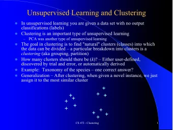
Unsupervised Learning Unsupervised Learning Learning without Class - PowerPoint PPT Presentation

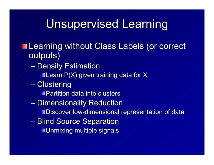
Unsupervised Learning Unsupervised Learning Learning without Class Labels (or correct Learning without Class Labels (or correct outputs) outputs) – Density Estimation Density Estimation – Learn P(X) given training data for X Learn P(X) given training data for X – Clustering Clustering – Partition data into clusters Partition data into clusters – Dimensionality Reduction Dimensionality Reduction – Discover low- -dimensional representation of data dimensional representation of data Discover low – Blind Source Separation Blind Source Separation – Unmixing multiple signals Unmixing multiple signals

Density Estimation Density Estimation Given: S = { x , x , … …, , x } Given: S = { 1 , 2 , N } x 1 x 2 x N Find: P( x ) Find: P( x ) Search problem: Search problem: ∑ i h ∑ argmax h P(S|h) = argmax h log P( x |h) argmax h P(S|h) = argmax i log P( i |h) x i

Unsupervised Fitting of Unsupervised Fitting of the Naï ïve Bayes Model ve Bayes Model the Na y … x 1 x 2 x 3 x n y is discrete with K values y is discrete with K values ∑ k ∏ j ) = ∑ P(y=k) ∏ P( x P(x j | y=k) P( x ) = k P(y=k) j P(x j | y=k) finite mixture model finite mixture model we can think of each y=k as a separate we can think of each y=k as a separate “cluster cluster” ” of data points of data points “

The Expectation- -Maximization Algorithm (1): Maximization Algorithm (1): The Expectation Hard EM Hard EM Learning would be easy if we knew Learning would be easy if we knew y i for each x y i for each x i y i y x i x i i i Idea: guess them and then Idea: guess them and then y 1 y x 1 x 1 1 iteratively revise our guesses to iteratively revise our guesses to y 2 y x 2 x 2 2 maximize P(S|h) maximize P(S|h) … … … … y N y x N x N N

Hard EM (2) Hard EM (2) 1. Guess initial Guess initial y y values to get values to get “ “complete complete 1. data” ” data y i y x i x i i 2. M Step: Compute probabilities for M Step: Compute probabilities for 2. y 1 y x 1 x hypotheses (model) from complete hypotheses (model) from complete 1 1 data [Maximum likelihood estimate of data [Maximum likelihood estimate of y 2 y x 2 x 2 2 the model parameters] the model parameters] … … … … 3. E Step: Classify each example using E Step: Classify each example using 3. y N y x N x N N the current model to get a new y y value value the current model to get a new [Most likely class ŷ ŷ of each example] of each example] [Most likely class 4. Repeat steps 2 Repeat steps 2- -3 until convergence 3 until convergence 4.

Special Case: k- -Means Clustering Means Clustering Special Case: k 1. Assign an initial Assign an initial y y i to each data point x at i to each data point i at 1. x i random random 2. M Step. For each class k = 1, M Step. For each class k = 1, … …, K , K 2. compute the mean: compute the mean: µ k ∑ i µ k ∑ = 1/N k · I[y I[y i = k] k = 1/N i = k] x i i · i x 3. E Step. For each example x E Step. For each example x i , assign it to i , assign it to 3. the class k with the nearest mean: the class k with the nearest mean: - µ µ k y i = argmin k || x || y i = argmin k || i - k || x i 4. Repeat steps 2 and 3 to convergence Repeat steps 2 and 3 to convergence 4.

Gaussian Interpretation of K- -means means Gaussian Interpretation of K Each feature x j in class k is gaussian Each feature x j in class k is gaussian µ kj distributed with mean µ and constant distributed with mean kj and constant σ 2 variance σ 2 variance " # ( k x j − µ kj k ) 2 1 − 1 P ( x j | y = k ) = √ exp σ 2 2 2 πσ k x j − µ kj k 2 = − 1 log P ( x j | y = k ) + C σ 2 2 k x − µ kj k 2 = argmin argmax P ( x | y = k ) = argmax log P ( x | y ) = argmin k x − µ kj k y y y y This could easily be extended to have This could easily be extended to have Σ or class general covariance matrix Σ or class- - general covariance matrix Σ k specific Σ specific k

The EM algorithm The EM algorithm The true EM algorithm augments The true EM algorithm augments the incomplete data with a the incomplete data with a probability distribution over the probability distribution over the y i y x i x i i possible y y values values possible P(y 1 P(y 1 ) ) x 1 x 1 P(y 2 P(y 2 ) ) x 2 x 1. Start with initial naive Bayes Start with initial naive Bayes 2 1. hypothesis hypothesis … … … … 2. E step E step: : For each example, compute For each example, compute 2. P(y N P(y N ) ) x N x N P(y i ) and add it to the table P(y i ) and add it to the table 3. M step: Compute updated estimates M step: Compute updated estimates 3. of the parameters of the parameters 4. Repeat steps 2 Repeat steps 2- -3 to convergence. 3 to convergence. 4.

Details of the M step Details of the M step Each example x is treated as if y i =k with Each example i is treated as if y i =k with x i probability P(y i =k | x ) probability P(y i =k | i ) x i N X 1 P ( y = k ) := P ( y i = k | x i ) N i =1 P i P ( y i = k | x i ) · I ( x ij = v ) P ( x j = v | y = k ) := P N i =1 P ( y i = k | x i )

Example: Mixture of 2 Gaussians Example: Mixture of 2 Gaussians Initial distributions means at -0.5, +0.5

Example: Mixture of 2 Gaussians Example: Mixture of 2 Gaussians Iteration 1

Example: Mixture of 2 Gaussians Example: Mixture of 2 Gaussians Iteration 2

Example: Mixture of 2 Gaussians Example: Mixture of 2 Gaussians Iteration 3

Example: Mixture of 2 Gaussians Example: Mixture of 2 Gaussians Iteration 10

Example: Mixture of 2 Gaussians Example: Mixture of 2 Gaussians Iteration 20

Evaluation: Test set likelihood Evaluation: Test set likelihood Overfitting is also a problem in unsupervised Overfitting is also a problem in unsupervised learning learning

Potential Problems Potential Problems σ k If σ is allowed to vary, it may go to zero, If k is allowed to vary, it may go to zero, which leads to infinite likelihood which leads to infinite likelihood σ Fix by placing an overfitting penalty on 1/ σ Fix by placing an overfitting penalty on 1/

Choosing K Choosing K Internal holdout likelihood Internal holdout likelihood

Unsupervised Learning for Unsupervised Learning for Sequences Sequences Suppose each training example X is a Suppose each training example i is a X i sequence of objects: sequence of objects: = ( x , x , … …, , x ) i = ( i1 , i2 , i ) X i x i1 x i2 x i,T X i,Ti Fit HMM by unsupervised learning Fit HMM by unsupervised learning 1. Initialize model parameters Initialize model parameters 1. 2. E step: apply forward E step: apply forward- -backward algorithm to backward algorithm to 2. estimate P(y it | X ) at each point t estimate P(y it | i ) at each point t X i 3. M step: estimate model parameters M step: estimate model parameters 3. 4. Repeat steps 2 Repeat steps 2- -3 to convergence 3 to convergence 4.

Agglomerative Clustering Agglomerative Clustering Initialize each data point to be its own cluster Initialize each data point to be its own cluster Repeat: Repeat: – Merge the two clusters that are most similar Merge the two clusters that are most similar – – Build dendrogram with height = distance between the most similar Build dendrogram with height = distance between the most similar clusters clusters – Apply various intuitive methods to choose number of clusters Apply various intuitive methods to choose number of clusters – – Equivalent to choosing where to Equivalent to choosing where to “ “slice slice” ” the dendrogram the dendrogram Source: Charity Morgan http://www.people.fas.harvard.edu/~rizem/teach/stat325/CharityCluster.ppt

Agglomerative Clustering Agglomerative Clustering Each cluster is defined only by the points it Each cluster is defined only by the points it contains (not by a parameterized model) contains (not by a parameterized model) Very fast (using priority queue) Very fast (using priority queue) No objective measure of correctness No objective measure of correctness Distance measures Distance measures – distance between nearest pair of points distance between nearest pair of points – – distance between cluster centers distance between cluster centers –

Probabilistic Agglomerative Clustering Probabilistic Agglomerative Clustering = Bottom- -up Model Merging up Model Merging = Bottom Each data point is an initial cluster but with Each data point is an initial cluster but with σ k penalized σ penalized k Repeat: Repeat: – Merge the two clusters that would most Merge the two clusters that would most – increase the penalized log likelihood increase the penalized log likelihood – Until no merger would further improve Until no merger would further improve – likelihood likelihood σ k Note that without the penalty on σ , the Note that without the penalty on k , the algorithm would never merge anything algorithm would never merge anything