Introduction to PCA Unsupervised Learning in R Unsupervised - PowerPoint PPT Presentation
UNSUPERVISED LEARNING IN R Introduction to PCA Unsupervised Learning in R Unsupervised learning Two methods of clustering finding groups of homogeneous items Next up, dimensionality reduction Find structure in features
UNSUPERVISED LEARNING IN R Introduction to PCA
Unsupervised Learning in R Unsupervised learning ● Two methods of clustering — finding groups of homogeneous items ● Next up, dimensionality reduction ● Find structure in features ● Aid in visualization
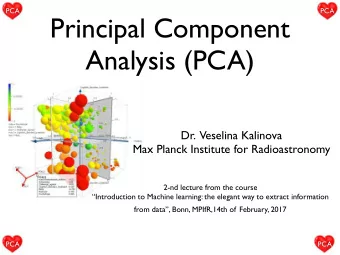
Unsupervised Learning in R Dimensionality reduction ● A popular method is principal component analysis (PCA) ● Three goals when finding lower dimensional representation of features: ● Find linear combination of variables to create principal components ● Maintain most variance in the data ● Principal components are uncorrelated (i.e. orthogonal to each other)
Unsupervised Learning in R PCA intuition 2 dimensions: x and y PCA 1 dimension: One principal component
Unsupervised Learning in R PCA intuition Regression line represents the principal component
Unsupervised Learning in R PCA intuition Projected values on principal component is called component scores or factor scores
Unsupervised Learning in R Visualization of high dimensional data Three-dimensional ? Two-dimensional Four-dimensional
Unsupervised Learning in R Visualization PC1 maintains 92% of the variability of original data
Unsupervised Learning in R PCA in R > pr.iris <- prcomp(x = iris[-5], scale = FALSE, center = TRUE) > summary(pr.iris) Importance of components: PC1 PC2 PC3 PC4 Standard deviation 2.0563 0.49262 0.2797 0.15439 Proportion of Variance 0.9246 0.05307 0.0171 0.00521 Cumulative Proportion 0.9246 0.97769 0.9948 1.00000
UNSUPERVISED LEARNING IN R Let’s practice!
UNSUPERVISED LEARNING IN R Visualizing and interpreting PCA results
Unsupervised Learning in R Biplot Shows that Petal.Width and Petal.Length are correlated in the original data
Unsupervised Learning in R Scree plot When number of PCs and number of original features are the same, the cumulative proportion of variance explained is 1
Unsupervised Learning in R Biplots and scree plots in R > # Creating a biplot > pr.iris <- prcomp(x = iris[-5], scale = FALSE, center = TRUE) > biplot(pr.iris) > # Getting proportion of variance for a scree plot > pr.var <- pr.iris$sdev^2 > pve <- pr.var / sum(pr.var) > # Plot variance explained for each principal component > plot(pve, xlab = "Principal Component", ylab = "Proportion of Variance Explained", ylim = c(0, 1), type = "b")
Unsupervised Learning in R Biplots and scree plots in R Biplot Scree plot
UNSUPERVISED LEARNING IN R Let’s practice!
UNSUPERVISED LEARNING IN R Practical issues with PCA
Unsupervised Learning in R Practical issues with PCA ● Scaling the data ● Missing values: ● Drop observations with missing values ● Impute / estimate missing values ● Categorical data: ● Do not use categorical data features ● Encode categorical features as numbers
Unsupervised Learning in R Scaling > data(mtcars) > head(mtcars) mpg cyl disp hp drat wt qsec vs am gear carb Mazda RX4 21.0 6 160 110 3.90 2.620 16.46 0 1 4 4 Mazda RX4 Wag 21.0 6 160 110 3.90 2.875 17.02 0 1 4 4 Datsun 710 22.8 4 108 93 3.85 2.320 18.61 1 1 4 1 Hornet 4 Drive 21.4 6 258 110 3.08 3.215 19.44 1 0 3 1 Hornet Sportabout 18.7 8 360 175 3.15 3.440 17.02 0 0 3 2 Valiant 18.1 6 225 105 2.76 3.460 20.22 1 0 3 1 # Means and standard deviations vary a lot > round(colMeans(mtcars), 2) mpg cyl disp hp drat wt qsec vs am gear carb 20.09 6.19 230.72 146.69 3.60 3.22 17.85 0.44 0.41 3.69 2.81 > round(apply(mtcars, 2, sd), 2) mpg cyl disp hp drat wt qsec vs am gear carb 6.03 1.79 123.94 68.56 0.53 0.98 1.79 0.50 0.50 0.74 1.62
Unsupervised Learning in R Importance of scaling data
Unsupervised Learning in R Scaling and PCA in R > prcomp(x, center = TRUE, scale = FALSE)
UNSUPERVISED LEARNING IN R Let’s practice!
UNSUPERVISED LEARNING IN R Additional uses of PCA and wrap-up
Unsupervised Learning in R Dimensionality reduction
Unsupervised Learning in R Data visualization
Unsupervised Learning in R Interpreting PCA results
Unsupervised Learning in R Importance of data scaling
Unsupervised Learning in R Up next # URL to cancer dataset hosted on DataCamp servers > url <- "http://s3.amazonaws.com/assets.datacamp.com/production/ course_1903/datasets/WisconsinCancer.csv" # Download the data: wisc.df > wisc.df <- read.csv(url) > wisc.data[1:6, 1:5] radius_mean texture_mean perimeter_mean area_mean smoothness_mean 842302 17.99 10.38 122.80 1001.0 0.11840 842517 20.57 17.77 132.90 1326.0 0.08474 84300903 19.69 21.25 130.00 1203.0 0.10960 84348301 11.42 20.38 77.58 386.1 0.14250 84358402 20.29 14.34 135.10 1297.0 0.10030 843786 12.45 15.70 82.57 477.1 0.12780
UNSUPERVISED LEARNING IN R Let’s practice!
Recommend
More recommend
Explore More Topics
Stay informed with curated content and fresh updates.
