Principal Component Analysis (PCA) Dr. Veselina Kalinova Max - PowerPoint PPT Presentation

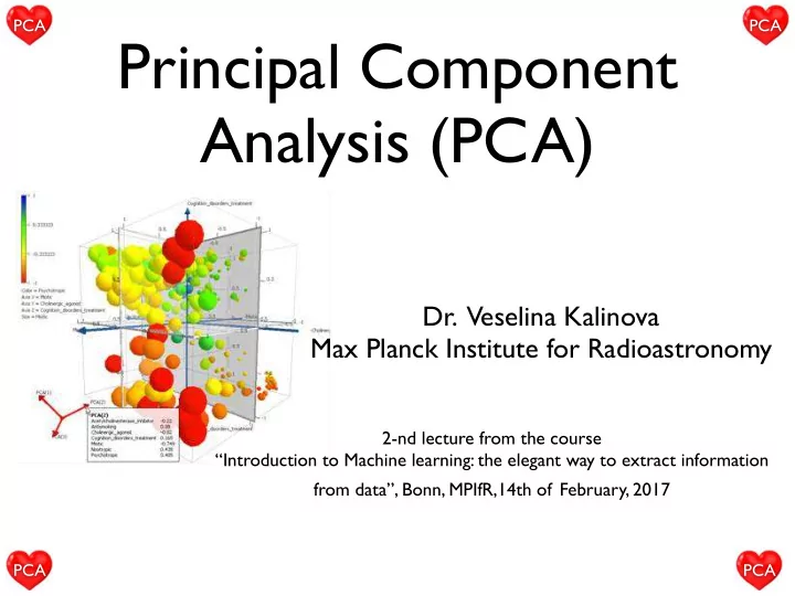
PCA PCA Principal Component Analysis (PCA) Dr. Veselina Kalinova Max Planck Institute for Radioastronomy 2-nd lecture from the course “Introduction to Machine learning: the elegant way to extract information from data”, Bonn, MPIfR,14th of February, 2017 PCA PCA

Machine Learning - PCA PCA the elegant way to extract information from complex and multi-dimensional data Math matters ! credit: IBM Data Science Experience PCA PCA http://datascience.ibm.com/blog/the-mathematics-of-machine-learning/

Principal Component Analysis (PCA) PCA PCA Motivation Which projection do you think is better to get more information from the data? It’s the projection that maximises the area of the shadow and an equivalent measurement is the sums of squares of the distances between points in the projection, we want to see as much of the variation as possible, that’s what PCA does. PCA PCA credit: http://web.stanford.edu/class/bios221/PCA_Slides.html

PCA Principal Component Analysis (PCA) PCA Definition Principal component analysis (PCA) is a statistical procedure that uses an orthogonal transformation to convert a set of observations of possibly correlated variables into a set of values of linearly uncorrelated variables called principal components. The number of principal components is less than or equal to the number of original Karl Pearson (1857 - 1936), variables. English mathematician and biostatistician, This transformation is defined in such a way Fig. PCA of a multivariate inventor of PCA in 1901 year. that the first principal component has the largest Gaussian distribution centered at (1,3) with a standard deviation of possible variance (that is, accounts for as much 3 in roughly the (0.866, 0.5) of the variability in the data as possible), and direction and of 1 in the each succeeding component in turn has the orthogonal direction. The vectors highest variance possible under the constraint shown are the eigenvectors of the that it is orthogonal to the preceding covariance matrix scaled by the components. square root of the corresponding eigenvalue, and shifted so their tails are at the mean. The resulting vectors are an uncorrelated orthogonal basis set. PCA PCA credit: Wikipedia

Method: I step Principal Component Analysis (PCA)- general idea 2-D case y PC1 PC2 PC2 y P C 1 x x PC1 captures the direction of the most variation PC2 captures the direction of the 2 nd most variation … PCn captures the direction of the n nd most variation (n=100 for our sample. However, we need only n=2 to reconstruct 99 % of the Vc data for all galaxies. )

PCA orthogonal base of eigenvectors original data set red lines represent the eigenvectors’ axes, i.e. PC axes oscillating around the main PC axes credit: http://stats.stackexchange.com/questions/2691/making-sense-of-principal-component-analysis-eigenvectors-eigenvalues

PCA on Images

PCA on Images: Eigenfaces Checks if the image is a face using PC space credit: http://archive.cnx.org/contents/ce6cf0ed-4c63-4237-b151-2f4eff8a7b8c@6/facial-recognition- using-eigenfaces-obtaining-eigenfaces

Happiness subspace (method A) Recognising emotions using PCA (eigenfaces) credit : Barnabás Póczos

Disgust subspace (method A) Recognising emotions using PCA (eigenfaces) credit : Barnabás Póczos

Representative male face per country

Representative female face per country

Compressing images using PCA

Original Image • Divide the original 372x492 image into patches: • Each patch is an instance that contains 12x12 pixels on a grid • View each as a 144-D vector credit : Barnabás Póczos 36

PCA compression: 144D ) 60D credit : Barnabás Póczos

PCA compression: 144D ) 16D 16 most important eigenvectors 2 2 2 2 4 4 4 4 6 6 6 6 8 8 8 8 1 0 1 0 1 0 1 0 1 2 1 2 1 2 1 2 2 4 6 8 1 0 1 2 2 4 6 8 1 0 1 2 2 4 6 8 1 0 1 2 2 4 6 8 1 0 1 2 2 2 2 2 4 4 4 4 6 6 6 6 8 8 8 8 1 0 1 0 1 0 1 0 1 2 1 2 1 2 1 2 2 4 6 8 1 0 1 2 2 4 6 8 1 0 1 2 2 4 6 8 1 0 1 2 2 4 6 8 1 0 1 2 2 2 2 2 4 4 4 4 6 6 6 6 8 8 8 8 1 0 1 0 1 0 1 0 1 2 1 2 1 2 1 2 2 4 6 8 1 0 1 2 2 4 6 8 1 0 1 2 2 4 6 8 1 0 1 2 2 4 6 8 1 0 1 2 2 2 2 2 4 4 4 4 6 6 6 6 8 8 8 8 1 0 1 0 1 0 1 0 1 2 1 2 1 2 1 2 2 4 6 8 1 0 1 2 2 4 6 8 1 0 1 2 2 4 6 8 1 0 1 2 2 4 6 8 1 0 1 2 PCA compression: 144D ) 3D 3 most important eigenvectors 2 2 4 4 6 6 8 8 1 0 1 0 1 2 1 2 2 4 6 8 1 0 1 2 2 4 6 8 1 0 1 2 2 4 6 8 1 0 1 2 2 4 6 8 1 0 1 2 credit : Barnabás Póczos

PCA compression: 144D ) 1D credit : Barnabás Póczos

PCA application to Astronomy

Application of PCA to Astronomy Different CVC due to different potential Kalinova et al., 2017, MNRAS, submitted

Application of PCA to Astronomy We compare the shapes of the rotation curves in each cell of the radius (x-axis). Kalinova et al., 2017, MNRAS, submitted

Application of PCA to Astronomy We compare the shape of the rotation curves in both axes - radius and velocity amplitude. Kalinova et al., 2017, MNRAS, submitted

Kalinova et al., 2017, MNRAS, submitted Principal Component Analysis (PCA): Reconstructing Vc Main PC Eigenvectors of V c Reconstructed V c via PCA 120 400 u 1 (93.33%) 100 NGC7671 350 Eigenvectors [km s -1 ] 80 300 60 V c [kms -1 ] 40 PC1= 1.29 PC4=-2.41 250 PC2=-2.50 PC5= 0.84 u 3 (0.87%) 20 PC3=-1.92 u 4 (0.29%) u 5 (0.07%) 200 0 u 2 (5.41%) -20 150 0.2 0.4 0.6 0.8 1.0 1.2 1.4 0.2 0.4 0.6 0.8 1.0 1.2 1.4 R/R e R/R e V c, rec = ( PC 1 u 1 + PC 2 u 2 + PC 3 u 3 + PC 4 u 4 + PC 5 u 5 )+ V c . mean velocity P C1 = +0.79, P C2 = − 1.86, PC3 = − 1.98, reconstructed of the sample PC4 = − 1.90, PC5 = +1.82.