PCA applied to bodies e 1 e 2 e 3 e 4 e 5 +4 4 Freifeld and - PowerPoint PPT Presentation
PCA: Principal Component Analysis Iain Murray http://iainmurray.net/ PCA: Principal Component Analysis Code assuming X is zero-mean 1 % Find top K principal directions: 0 [V, E] = eig(X*X); [E,id] = sort(diag(E),1,descend); 1 V
PCA: Principal Component Analysis Iain Murray http://iainmurray.net/
PCA: Principal Component Analysis Code assuming X is zero-mean 1 % Find top K principal directions: 0 [V, E] = eig(X’*X); [E,id] = sort(diag(E),1,’descend’); −1 V = V(:, id(1:K)); % DxK −1 0 1 % Project to K-dims: X_kdim = X*V; % NxK K = 1 + = X % Project back: · = Xproj X_proj = X_kdim * V’; % NxD — = V(:,1)
PCA applied to bodies e 1 e 2 e 3 e 4 e 5 +4 σ − 4 σ µ Freifeld and Black, ECCV 2012
PCA applied to DNA Novembre et al. (2008) — doi:10.1038/nature07331 Carefully selected both individuals and features 1,387 individuals 197,146 single nucleotide polymorphisms (SNPs) Each person reduced to two(!) numbers with PCA
MSc course enrollment data Binary S × C matrix M M sc = 1 , if student s taking course c Each course is a length S vector . . . OR each student is a length C vector
PCA applied to MSc courses CPSLP MT ANLP 0.3 NLU SProc ASR 0.2 TCM ALE1 CCS MASWS 0.1 CCN MI NC PA ST BIO1 BIO2 CNV DS PPLS 0 DAPA PM CN SEOC DIE SAPM IQC EXC ABS LP SP COPT HCI QSX TDD ADBS AR IJP CG CAV RC TTS NIP AGTA −0.1 IAML RLSC AV IT RSS DME DMR −0.2 RL MLPR PMR −0.2 −0.1 0 0.1 0.2
PCA applied to MSc students 0.1 0.05 0 −0.05 −0.1 −0.15 −0.04 −0.02 0 0.02 0.04 0.06 0.08 0.1 0.12 0.14 0.16
Truncated SVD % PCA via SVD, % for zero-mean X: [U, S, V] = svd(X, 0); X 11 X 12 X 1 D · · · U = U(:, 1:K); X 21 X 22 X 2 D · · · S = S(1:K, 1:K); X 31 X 32 X 3 D · · · V = V(:, 1:K); ≈ X_kdim = U*S; X 41 X 42 X 4 D · · · X_proj = U*S*V’; X 51 X 52 X 5 D · · · . . . ... . . . . . . X N 1 X N 2 X ND · · · U 11 U 1 K · · · U 21 U 2 K · · · S 11 V 11 V 21 V D 1 0 0 · · · U 31 U 3 K · · · . . . ... ... . . . U 41 U 4 K · · · . . . 0 0 U 51 U 5 K · · · S KK V 1 K V 2 K V DK 0 0 · · · . . ... . . . . U N 1 U NK · · · V ⊤ X ≈ U S
PCA summary Project data onto major axes of covariance X ⊤ X is covariance if make data zero mean Low-dim coordinates can be useful: — visualization — if can’t cope with high-dim data Can project back into original space: — detail is lost: still in K -dim subspace — PCA minimizes the square error
PPCA: Probabilistic PCA Gaussian model: Σ = WW ⊤ + σ 2 I W is D × K , σ 2 small ⇒ nearly low-rank W is also orthogonal As σ 2 → 0 , recover PCA. Need σ 2 > 0 to explain data Special case of factor analysis: Σ = WW ⊤ + Φ , with Φ diagonal
Dim reduction in other models Can replace x with A x in any model A is a K × D matrix of projection params Large D : a lot of extra parameters NB: Neural nets already have such projections
Practical tip Scale features to have unit variance Equivalently: find eigenvectors of correlation rather than covariance Avoids issues with (arbitrary?) scaling. If multiply feature by 10 9 , PC points along that feature E.g., if change unit of feature from metres to nanometres
Recommend
More recommend
Explore More Topics
Stay informed with curated content and fresh updates.
