12. Unsupervised Deep Learning CS 535 Deep Learning, Winter 2018 - PowerPoint PPT Presentation

Nov 28, 2022 •311 likes •1.48k views

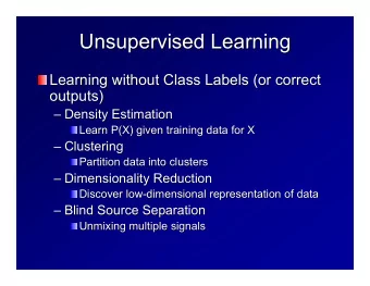
12. Unsupervised Deep Learning CS 535 Deep Learning, Winter 2018 Fuxin Li With materials from Wanli Ouyang, Zsolt Kira, Lawrence Neal, Raymond Yeh, Junting Lou and Teck-Yian Lim Unsupervised Learning in General Unsupervised learning is

Sliced Wasserstein Distance • For each image, build a Laplacian pyramid • Sample many patches from these pyramids • Normalize them by their mean/variance • Yields R/G/B histograms at each scale • Measures difference in distributions • Used as SWD(real_images, generated_images) • Lower score (more similarity) is better • Measures realism
Experiments
Nearest Neighbors Comparison with training set images
Results
Boltzmann Machine (Fully-connected MRF/CRF) • Undirected graphical model • Binary values on each variable • • • Consider only binary interactions    )     E ( x; w x x x ij i j i i  i j i   f ( x ; ) m m m    E ( x ; ) e f ( x ; )     P ( x ; ) m ,        E ( x ; ) f ( x ; ) e Z ( ) m m m x x m  w  : { , } ij i Boltzmann machine: � � � � �
Restricted Boltzmann Machines • We restrict the connectivity to make j hidden inference and learning easier. • Only one layer of hidden units. visible i • No connections between hidden units. 1  p ( h ) • In an RBM it only takes one step to  1 ( ) j reach thermal equilibrium when the    b v w visible units are clamped. j i ij  1 e  i vis • So we can quickly get the exact value of :   v i h j v
What you gain
Example: ShapeBM (Eslami et al. 2012) • Generating shapes • 2-layer RBM with local connections • Learning from many horses
Training: Contrastive divergence Start with a training vector on the j j visible units.  v i h j  0  v i h j  1 Update all the hidden units in parallel. i i Update the all the visible units in t = 0 t = 1 parallel to get a “ reconstruction ” . reconstruction data Update the hidden units again . D w ij  e (  v i h j  0   v i h j  1 ) This is not following the gradient of the log likelihood. But it works well.
28x28 Layerwise Pretraining T W 1 (Hinton & Salakhutdinov, 2006) 1000 neurons • They always looked like a really T W 2 nice way to do non-linear 500 neurons T dimensionality reduction: W 3 • But it is very difficult to 250 neurons T optimize deep autoencoders W 4 linear using backpropagation. 30 units • We now have a much better W 4 way to optimize them: 250 neurons • First train a stack of 4 RBM’s W 3 • Then “unroll” them. 500 neurons • Then fine-tune with backprop. W 2 1000 neurons W 1 28x28 100

Recommend

Unsupervised Deep Learning Tutorial - Part 2 Alex Graves MarcAurelio Ranzato

Unsupervised Deep Learning Tutorial - Part 2 Alex Graves MarcAurelio Ranzato gravesa@google.com ranzato@fb.com NeurIPS, 3 December 2018 Overview Practical Recipes of Unsupervised Learning Learning representations Learning to

1.16k views • 103 slides

UNSUPERVISED LEARNING, CLUSTERING UNSUPERVISED LEARNING UNSUPERVISED LEARNING Supervised

UNSUPERVISED LEARNING, CLUSTERING UNSUPERVISED LEARNING UNSUPERVISED LEARNING Supervised learning: X - y pairs, f(x) function approximation Unsupervised learning: only X, no y Exploring the space of X measurements,

440 views • 14 slides

Introduction to PCA Unsupervised Learning in R Unsupervised learning Two methods of

UNSUPERVISED LEARNING IN R Introduction to PCA Unsupervised Learning in R Unsupervised learning Two methods of clustering finding groups of homogeneous items Next up, dimensionality reduction Find structure in features

904 views • 29 slides

Unsupervised Learning and Inverse Problems with Deep Neural Networks J oan Bruna, Stphane

Unsupervised Learning and Inverse Problems with Deep Neural Networks J oan Bruna, Stphane Mallat, Ivan Dokmanic, Martin de Hoop cole Normale Suprieure www.di.ens.fr/data Deep Convolutional Networks ( x ) x ( u ) L j L 1 f M (

520 views • 47 slides

Unsupervised Deep Learning Tutorial Part 1 Alex Graves MarcAurelio Ranzato NeurIPS, 3

Unsupervised Deep Learning Tutorial Part 1 Alex Graves MarcAurelio Ranzato NeurIPS, 3 December 2018 Part 1 Alex Graves Introduction to unsupervised learning Autoregressive models Representation learning

1.47k views • 90 slides

3D Deep Clustering a clustering framework for unsupervised learning of 3D object feature

3D Deep Clustering a clustering framework for unsupervised learning of 3D object feature descriptors LAMBDA Workshop on Retrieval and Shape analysis Alexandros Georgiou M.Sc. in Algorithms, Logic and Discrete Mathematics 1/12 Problem

570 views • 53 slides

Deep-Learning: Unsupervised Generative models Deep Belief Networks Deep Stacked AutoEncoders

Deep-Learning: Unsupervised Generative models Deep Belief Networks Deep Stacked AutoEncoders Generative Adversarial Networks Pr. Fabien MOUTARDE Center for Robotics MINES ParisTech PSL Universit Paris Fabien.Moutarde@mines-paristech.fr

777 views • 23 slides

Unsupervised Video Object Segmentation for Deep Reinforcement Learning Authors: Vik Goel,

Unsupervised Video Object Segmentation for Deep Reinforcement Learning Authors: Vik Goel, Jameson Weng, Pascal Poupart Presenter: Siliang Huang Outline Problem tackled Solution proposed RL background Architecture and

857 views • 30 slides

Anomaly Detection and Categorization Using Unsupervised Deep Learning S6340 Thursday 7 th April

Anomaly Detection and Categorization Using Unsupervised Deep Learning S6340 Thursday 7 th April 2016 GPU Technology Conference A. Stephen McGough , Noura Al Moubayed, Jonathan Cumming, Eduardo Cabrera, Peter Matthews, Toby P . Breckon, Ed

599 views • 29 slides

A Hybrid Deep Learning Approach For Chaotic Time Series Prediction Based On Unsupervised Feature

A Hybrid Deep Learning Approach For Chaotic Time Series Prediction Based On Unsupervised Feature Learning Norbert Ayine Agana Advisor: Abdollah Homaifar Autonomous Control & Information Technology Institute (ACIT), Departmenent of

379 views • 35 slides

Current State of Unsupervised Deep Learning William Falcon, PhD Student AGENDA AGENDA

Current State of Unsupervised Deep Learning William Falcon, PhD Student AGENDA AGENDA Unsupervised vs self-supervised vs supervised learning Why we don't like supervised learning Cost of supervised learning Theoretical approaches to

846 views • 46 slides

From unsupervised induction of linguistic structures from text towards applications in deep

Alexander Panchenko From unsupervised induction of linguistic structures from text towards applications in deep learning In close collaboration with May 28, 2018 From unsupervised induction of linguistic structures to applications in deep

1.68k views • 142 slides

Unsupervised Learning and Clustering l In unsupervised learning you are given a data set with no

Unsupervised Learning and Clustering l In unsupervised learning you are given a data set with no output classifications (labels) l Clustering is an important type of unsupervised learning PCA was another type of unsupervised learning l The

858 views • 38 slides

Unsupervised Learning Unsupervised vs Supervised Learning: Most of this course focuses on

Unsupervised Learning Unsupervised vs Supervised Learning: Most of this course focuses on supervised learning methods such as regression and classification. In that setting we observe both a set of features X 1 , X 2 , . . . , X p for each

721 views • 60 slides

Unsupervised Learning Unsupervised vs Supervised Learning: Most of this course focuses on

934 views • 50 slides

Unsupervised Learning Andrea Passerini passerini@disi.unitn.it Machine Learning Unsupervised

Unsupervised Learning Andrea Passerini passerini@disi.unitn.it Machine Learning Unsupervised Learning Unsupervised Learning Setting Supervised learning requires the availability of labelled examples Labelling examples can be an extremely

752 views • 27 slides

8. Other Deep Architectures CS 519 Deep Learning, Winter 2018 Fuxin Li With materials from Zsolt

8. Other Deep Architectures CS 519 Deep Learning, Winter 2018 Fuxin Li With materials from Zsolt Kira and Ian Goodfellow A brief overview of other architectures Unsupervised Architectures Deep Belief Networks Autoencoders GANs

439 views • 25 slides

Unsupervised Deep Learning by Neighbourhood Discovery ICML-2019 Jiabo Huang 1 Qi Dong 1 Shaogang

Unsupervised Deep Learning by Neighbourhood Discovery ICML-2019 Jiabo Huang 1 Qi Dong 1 Shaogang Gong 1 Xiatian Zhu 2 1 Queen Mary University of London 2 Vision Semantic Ltd. Related Works & Motivation Related Works Clustering

535 views • 20 slides

Machine Learning for NLP Unsupervised Learning Aurlie Herbelot 2019 Centre for Mind/Brain

Machine Learning for NLP Unsupervised Learning Aurlie Herbelot 2019 Centre for Mind/Brain Sciences University of Trento 1 Unsupervised learning In unsupervised learning, we learn without training data. The idea is to find a

998 views • 67 slides

Deep Learning: Intro Juhan Nam Review of Traditional Machine Learning The traditional machine

GCT634/AI613: Musical Applications of Machine Learning (Fall 2020) Deep Learning: Intro Juhan Nam Review of Traditional Machine Learning The traditional machine learning pipeline Temporal Frame-level Unsupervised Classifier Summary

613 views • 27 slides

Unsupervised Learning Introduction Nakul Verma Unsupervised Learning What can we learn from

Unsupervised Learning Introduction Nakul Verma Unsupervised Learning What can we learn from data when label information is not available? Supervised learning framework Supervised learning Data: Assumption: there is a (relatively simple)

442 views • 16 slides

Unsupervised Visual Representation Learning by Context Prediction Berkan Demirel Most slides in

Unsupervised Visual Representation Learning by Context Prediction Berkan Demirel Most slides in this representation are adopted from authors' original presentation at ICCV 2015 ImageNet + Deep Learning Beagle - Image Retrieval - Detection

2.18k views • 33 slides

Representation Learning Lecture slides for Chapter 15 of Deep Learning www.deeplearningbook.org

Representation Learning Lecture slides for Chapter 15 of Deep Learning www.deeplearningbook.org Ian Goodfellow 2017-10-03 Unsupervised Pretraining Usually Hurts but Sometimes Helps Harm done by pretraining (Ma et al, 2015) Average advantage

586 views • 12 slides

Practical Unsupervised Learning INFO/CS 4300, Spring 2016 Jack Hessel Unsupervised Learning is

Practical Unsupervised Learning INFO/CS 4300, Spring 2016 Jack Hessel Unsupervised Learning is Cool! But how can we use this in our projects? 1. 2. But first, lets look at our dataset... Data Dimensionality! Probability of Lung Cancer

999 views • 55 slides