About this class Point Estimators The next two lectures are really - PowerPoint PPT Presentation

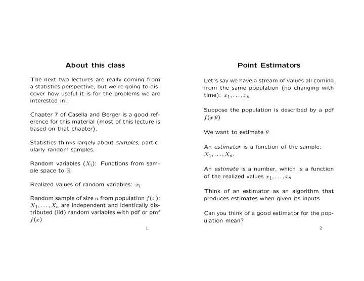
About this class Point Estimators The next two lectures are really coming from Let’s say we have a stream of values all coming a statistics perspective, but we’re going to dis- from the same population (no changing with cover how useful it is for the problems we are time): x 1 , . . . , x n interested in! Suppose the population is described by a pdf Chapter 7 of Casella and Berger is a good ref- f ( x | θ ) erence for this material (most of this lecture is based on that chapter). We want to estimate θ Statistics thinks largely about samples , partic- An estimator is a function of the sample: ularly random samples. X 1 , . . . , X n . Random variables ( X i ): Functions from sam- An estimate is a number, which is a function ple space to R of the realized values x 1 , . . . , x n Realized values of random variables: x i Think of an estimator as an algorithm that Random sample of size n from population f ( x ): produces estimates when given its inputs X 1 , . . . , X n are independent and identically dis- tributed (iid) random variables with pdf or pmf Can you think of a good estimator for the pop- f ( x ) ulation mean? 1 2

Maximum Likelihood Maximum Likelihood For a sample x = x 1 , . . . , x n let ˆ θ ( x ) be the pa- rameter value at which L ( θ | x ) attains its max- Method for deriving estimators. imum (as a function of θ , with x held fixed). Let x denote a realized random sample Then ˆ θ ( x ) is the maximum likelihood estimate ˆ of θ based on the realized sample x . θ ( X ) Likelihood function: is the maximum likelihood estimator based on n the sample X . � L ( θ | x ) = L ( θ | x 1 , . . . , x n ) = f ( x i | θ ) i =1 Note that the MLE has the same range as the parameter, by definition If X is discrete, L ( θ | x ) = P θ ( X = x ) Potential problems Intuitively, if L ( θ 1 | x ) > L ( θ 2 | x ) then θ 1 is in some ways a more plausible value for θ than is θ 2 • How to find and verify the maximum of the function? Can be generalized to multiple parameters θ 1 , . . . , θ n • Numerical sensitivity 3 4

Normal MLE Suppose X 1 , . . . , X n are iid N ( θ , 1) Di ff erentiable Likelihood Functions n 1 2 π e − 1 2 ( x i − θ ) 2 � L ( θ | x ) = √ i =1 Possible candidates are the values of θ 1 , . . . θ k that solve: Standard trick: work with the log likelihood ∂ L ( θ | x ) = 0 , ( i = 1 , . . . , k ) ∂θ i n 1 − 1 Must check whether any such value of θ is in 2( x i − θ ) 2 � log L ( θ | x ) = √ fact a global maximum (could be a minimum, 2 π i =1 an inflection point, a local maximum, and the boundary needs to be checked). Take the derivative, etc... n d 1 � d θ log L ( θ | x ) = √ ( x i − θ ) 2 π i =1 5 6

Bernoulli MLE Let X 1 , . . . , X n be iid Bernoulli( p ) d d θ log L ( θ | x ) = 0 n � n ( x i − θ ) = 0 ⇒ p x i (1 − p ) 1 − x i � L ( p | x ) = i =1 i =1 The only zero of this is for ˆ θ = x = p y (1 − p ) n − y where y = � x i To show that this is, in fact, the maximum likelihood estimate: 1. Show it is a maximum: log L ( p | x ) = y log p + ( n − y ) log(1 − p ) d 2 1 d θ 2 log L ( θ | x ) = 2 π ( − n ) < 0 √ If 0 < y < n dp log L ( p | x ) = y 1 d 1 p − ( n − y ) 2. Unique interior extremum, and a maximum 1 − p – therefore a global maximum dp log L ( p | x ) = 0 ⇒ 1 − p d = n − y p y 7

Binomial MLE, Unknown Number of Trials Population is binomial ( k, p ) with known p and unknown k n � k p = y Then ˆ � p x i (1 − p ) k − x i � n L ( k | x , p ) = x i i =1 Verify the maximum, and consider separately the cases where y = 0 (log likelihood is n log(1 − Maximizing by the di ff erentiation approach is p ) and y = n (log likelihood is n log p ) tricky k ≥ max x i i L ( k | x , p ) > L ( k − 1 | x , p ) L ( k | x , p ) > L ( k + 1 | x , p ) 8

MLE Instability L ( k − 1 | x , p ) = ( k (1 − p )) n L ( k | x , p ) Olkin, Petkau and Zidek [JASA 1981] give the � n i =1 ( k − x i ) following example. Suppose you are estimating the parameters for Conditions for a maximum are: a binomial ( k, p ) distribution (both k and p un- n known) and have the following data: ( k (1 − p )) n ≥ � ( k − x i ) i =1 16 , 18 , 22 , 25 , 27 and n Turns out the ML estimate of k is 99. (( k + 1)(1 − p )) n < � ( k + 1 − x i ) i =1 Question – what do you think the ML estimate of p is? Solution: Solve the equation: But what if the data were slightly noisy, and n (1 − p ) n = � (1 − x i z ) the 27 should have been a 28? i =1 for 0 ≤ z ≤ max i x i . Call this ˆ z The ML estimate of k is now 190! What’s going on here? Most likely the likeli- ˆ k is the largest integer equal to or less than hood function is very flat in the neighborhood 1 / ˆ z of the maximum 9

Bayesian Estimators Classical vs. Bayesian approach to statistics Classical: θ is an unknown but fixed parameter Bayesian: θ is a quantity described by a distri- Where m ( x ) is the marginal distribution of x , bution � f ( x | θ ) π ( θ ) d θ Prior distribution describes ones beliefs about The posterior distribution can be used to make θ before any data is seen statements about θ , but it’s still a distribution! For example, could use the mean of this dis- A sample is taken and the prior is then updated tribution as a point estimate of θ . to take the data into account, leading to a posterior distribution Let the prior be π ( θ ) and the sampling distri- bution be f ( x | θ ). Then the posterior is given by π ( θ | x ) = f ( x | θ ) π ( θ ) /m ( x ) 10

Binomial Bayes Estimation Let X 1 , . . . , X n be iid Bernoulli( p ) Let Y = � X i Suppose the prior distribution on p is beta( α , β ) (really, I should subscript these, but for nota- tional convenience I won’t...) Brief recap on the beta distribution – family of continuous distributions defined on [0 , 1] and Probability density function governed by the two shape parameters. Γ ( α + β ) Γ ( α ) Γ ( β ) x α − 1 (1 − x ) β − 1 A picture from wikipedia... α Nice fact: Mean is α + β 11

� n � p y (1 − p ) n − y f ( y | p ) = y π ( p ) = Γ ( α + β ) Γ ( α ) Γ ( β ) p α − 1 (1 − p ) β − 1 � 1 f ( y ) = 0 f ( y | p ) f ( p ) dp Bayes estimate combines prior information with � 1 � Γ ( α + β ) the data. � n Γ ( α ) Γ ( β ) p y + α − 1 (1 − p ) n − y + β − 1 dp = y 0 If we want to use a single number, we could use � Γ ( α + β ) � n Γ ( y + α ) Γ ( n − y + β ) = the mean of the posterior distribution, given by y Γ ( α ) Γ ( β ) Γ ( n + α + β ) y + α n + α + β Then the posterior distribution is given by f ( y | p ) π ( p ) f ( y ) Γ ( n + α + β ) Γ ( y + α ) Γ ( n − y + β ) p y + α − 1 (1 − p ) n − y + β − 1 = which is Beta( y + α , n − y + β ) !

Normal MLE when µ and σ Are Both Unknown n ( x i − θ ) 2 log L ( θ , σ 2 | x ) = − n 2 log(2 π ) − n 2 log σ 2 − 1 � σ 2 2 i =1 Partial derivatives: n ∂θ log L ( θ , σ 2 | x ) = 1 ∂ � ( x i − θ ) σ 2 i =1 n ∂σ 2 log L ( θ , σ 2 | x ) = − n 1 ∂ ( x i − θ ) 2 � 2 σ 2 + 2 σ 4 i =1 Setting to 0 and solving gives us: ˆ θ = x n σ 2 = 1 ( x i − x ) 2 � ˆ n i =1 12