Probabilistic reasoning over time - Hidden Markov Models (recap - PowerPoint PPT Presentation

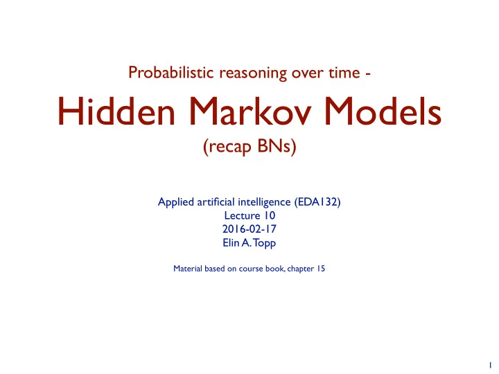
Probabilistic reasoning over time - Hidden Markov Models (recap BNs) Applied artificial intelligence (EDA132) Lecture 10 2016-02-17 Elin A. Topp Material based on course book, chapter 15 1

A robot’s view of the world... 9000 Scan data Robot 8000 Distance in mm relative to robot position 7000 6000 5000 4000 3000 2000 1000 0 − 1000 − 5000 − 4000 − 3000 − 2000 − 1000 0 1000 2000 3000 Distance in mm relative to robot position 2

Bayes’ Rule and conditional independence ℙ ( PersonLeg | #pointsInRange ∧ curvatureCorrect) = α ℙ ( #pointsInRange ∧ curvatureCorrect | PersonLeg) ℙ ( PersonLeg) = α ℙ ( #pointsInRange | PersonLeg) ℙ ( curvatureCorrect | PersonLeg) ℙ ( PersonLeg) An example of a naive Bayes model: ℙ ( Cause, Effect 1, ...., Effect n ) = ℙ ( Cause) ∏ i ℙ ( Effect i | Cause) Person leg Cause . . . #Points Curvature Effect 1 Effect n The total number of parameters is linear in n 3

Bayesian networks A simple, graphical notation for conditional independence assertions and hence for compact specification of full joint distributions Syntax: a set of nodes, one per random variable a directed, acyclic graph (link ≈ “directly influences”) a conditional distribution for each node given its parents: P ( X i | Parents( X i )) In the simplest case, conditional distribution represented as a conditional probability table ( CPT) giving the distribution over X i for each combination of parent values 4

Tracking and associating... while moving ... 5000 5000 Target 3 Target 0 Target 4 Target 1 Distance in mm relative to robot start position Distance in mm relative to robot start position Robot (1) Target 2 4000 4000 Robot Robot Robot (1) Robot (2) 3000 3000 2000 2000 1000 1000 0 0 − 1000 − 1000 − 1000 0 1000 2000 3000 4000 5000 − 1000 0 1000 2000 3000 4000 5000 Distance in mm relative to robot start position Distance in mm relative to robot start position 5000 Target 5 Target 6 Distance in mm relative to robot start position Target 7 4000 Target 8 Robot (1) Robot 3000 2000 1000 0 − 1000 − 1000 0 1000 2000 3000 4000 5000 Distance in mm relative to robot start position 5

Probabilistic reasoning over time ... means to keep track of the current state of - a process (temperature controller, other controllers) - an agent with respect to the world (localisation of a robot in some “world”) in order to make predictions or to simply understand what might have caused this current state. This involves both a transition model (how the state is assumed to change) and a sensor model (how observations / percepts are related to the world state). Previously: the focus was on what was possible to happen (e.g., search), now it is on what is likely / unlikely to happen the focus was on static worlds (Bayesian networks), now we look at dynamic processes where everything (state AND observations) depend on time. 6

Three classes of approaches Hidden Markov models (Particle filters) Kalman filters Dynamic Bayesian networks (cover actually the other two as special cases) But first, some basics ... 7

Reasoning over time With X t the current state description at time t E t the evidence obtained at time t we can describe a state transition model and a sensor model that we can use to model a time step sequence - a chain of states and sensor readings according to discrete time steps - so that we can understand the ongoing process. We assume to start out in X 0 , but evidence will only arrive after the first state transition is made: E 1 is then the first piece of evidence to be plugged into the chain. The “general” transition model would then specify ℙ ( X t | X 0:t-1 ) ... this would mean we need full joint distributions over all time steps... or not? X

The Markov assumption A process is Markov (i.e., complies with the Markov assumption), when any given state X t depends only on a finite and fixed number of previous states. X t –2 X t –1 X t X t +1 X t +2 (a) X t –2 X t –1 X t X t +1 X t +2 (b) 8

A first-order Markov chain as Bayesian network R t-1 P(R t | R t-1 ) T 0.7 F 0.3 “cause” / state Rain t-1 Rain t Rain t+1 Umbrella t-1 Umbrella t Umbrella t+1 “effect” / evidence R t P(U t | R t ) T 0.9 F 0.2 9

Inference for any t With ℙ ( X 0 ) the prior probability distribution in t=0 (i.e., the initial state model ), ℙ ( X i | X i-1 ) the state transition model and ℙ ( E i | X i ) the sensor model we have the complete joint distribution for all variables for any t. t ℙ ( X 0:t, E 1:t ) = ℙ ( X 0 ) ∏ ℙ ( X i | X i-1 ) ℙ ( E i | X i ) i=1 X

The Markov assumption First-order Markov chain: State variables (at t) contain ALL information needed for t+1. Sometimes, that is too strong an assumption (or too weak in some sense). Hence, increase either the order (second-order Markov chain) or add information into the state variable(s) ( R could include also Season , Humidity , Pressure , Location , instead of only “ Rain ”) Note: It is possible to express an increase in order by increasing the number of state variables, keeping the order fixed - for the umbrella world you could use R = <RainYesterday, RainToday> When things get too complex, rather add another sensor (e.g., observe coats). X

Inference in temporal models - what can we use all this for? • Filtering : Finding the belief state , or doing state estimation , i.e., computing the posterior distribution over the most recent state , using evidence up to this point: 
 ℙ ( X t | e 1:t ) • Predicting : Computing the posterior over a future state, using evidence up to this point: ℙ ( X t+k | e 1:t ) for some k>0 (can be used to evaluate course of action based on predicted outcome) • Smoothing : Computing the posterior over a past state, i.e., understand the past, given information up to this point: ℙ ( X k | e 1:t ) for some k with 0 ≤ k < t • Explaining : Find the best explanation for a series of observations, i.e., computing 
 argmax x 1:t P( x 1:t | e 1:t ) - can be efficiently handled by Viterbi algorithm • Learning : If sensor and / or transition model are not known, they can be learned from observations (by-product of inference in Bayesian network - both static or dynamic). Inference gives estimates, estimates are used to update the model, updated models provide new estimates (by inference). Iterate until converging - again, this is an instance of the EM-algorithm. 10


 
 Filtering: Prediction & update (FORWARD-step) ℙ ( X t+1 | e 1:t+1 ) = f( ℙ ( X t | e 1:t ), e t+1 ) = f 1:t+1 = ℙ ( X t+1 | e 1:t , e t+1 ) (decompose) = α ℙ ( e t+1 | X t+1 , e 1:t ) ℙ ( X t+1 | e 1:t ) (Bayes’ Rule) = α ℙ ( e t+1 | X t+1 ) ℙ ( X t+1 | e 1:t ) (1. Markov assumption (sensor model), 
 2. one-step prediction) = α ℙ ( e t+1 | X t+1 ) ∑ ℙ ( X t+1 | x t , e 1:t ) P( x t | e 1:t ) (sum over atomic events for X ) 
 x t = α ℙ ( e t+1 | X t+1 ) ∑ ℙ ( X t+1 | x t ) P( x t | e 1:t ) (Markov assumption) 
 x t ℙ ( X t | e 1:t ) (“forward message”, propagated recursively 
 f 1:t+1 = α FORWARD( f 1:t , e t+1 ) through “forward step function”) f 1:0 = ℙ ( X 0 ) 11

Prediction - filtering without the update ℙ ( X t+k+1 | e 1:t ) = ∑ ℙ ( X t+k+1 | x t ) P( x t+k | e 1:t ) (k-step prediction) 
 x t+k For large k the prediction gets quite blurry and will eventually converge into a stationary distribution at the mixing point , i.e., the point in time when this convergence is reached - in some sense this is when “everything is possible”. 
 12


 Smoothing: “explaining” backward ℙ ( X k | e 1:t ) = fb( X k, e 1:k , ℙ ( e k+1:t | X k )) with 0 ≤ k < t (understand the past from the 
 recent past) = ℙ ( X k | e 1:k , e k+1:t ) (decompose) = α ℙ ( X k | e 1:k ) ℙ ( e k+1:t | X k , e 1:k ) (Bayes’ Rule) = α ℙ ( X k | e 1:k ) ℙ ( e k+1:t | X k ) (Markov assumption) = α f 1:k ⨯ b k+1:t (forward-message ⨯ backward-message) 13


 
 Smoothing: calculating backward message b k+1:t = ℙ ( e k+1:t | X k ) = ∑ ℙ ( e k+1:t | X k , x k+1 ) ℙ ( x k+1 | X k ) (conditioning on X k+1 , i.e., looking “backward”) 
 x k+1 = ∑ P( e k+1:t | x k+1 ) ℙ ( x k+1 | X k ) (cond. indep. - Markov assumption) 
 x k+1 = ∑ P( e k+1 , e k+2:t | x k+1 ) ℙ ( x k+1 | X k ) (decompose) 
 x k+1 = ∑ P( e k+1 | x k+1 ) P( e k+2:t | x k+1 ) ℙ ( x k+1 | X k ) (1. sensor, 2. backward msg, 3. transition model) 
 x k+1 = BACKWARD( b k+2:t, e k+1 ) ℙ ( e k+1:t | X k ) (“backward message”, propagated recursively) 
 b k+1:t = BACKWARD( b k+2:t , e k+1 ) (through “backward step function”) b t+1:t = ℙ ( e t+1:t | X t ) = ℙ ( | X t ) = 1 14

Smoothing “in a nutshell”: Forward-Backward-algorithm ℙ ( X k | e 1:t ) = fb( e 1:k , ℙ ( e k+1:t | X k )) with 0 ≤ k < t understand the past from the 
 recent past = α f 1:k ⨯ b k+1:t by first filtering (forward) until step k , then 
 explaining backward from t to k+1 Obviously, it is a good idea to store the filtering (forward) results for later smoothing Drawback of the algorithm: not really suitable for online use ( t is growing, ...) Consequently, try with fixed-lag-smoothing (keeping a fixed-length window, BUT: “simple” Forward-Backward does not really do it efficiently - here we need HMMs) 15